Page 99 - Elements of Distribution Theory

P1: JZP
052184472Xc03 CUNY148/Severini May 24, 2005 2:34

3.3 Further Properties of Characteristic Functions 85

function of this distribution function is
2
σ 2
ϕ(t) = exp − t + iµt , ∞ < t < ∞.
2
Note that
√
∞ ∞
σ 2 (2π)
2
|ϕ(t)|≤ exp − t dt = ;
2 σ
−∞ −∞
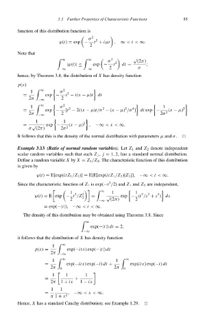
hence, by Theorem 3.8, the distribution of X has density function
p(x)
1 ∞ σ 2 2
= exp − t − i(x − µ)t dt
2π 2
−∞
1 ∞ σ 2 2 2 2 4 1 2
= exp − [t − 2i(x − µ)t/σ − (x − µ) /σ ] dt exp − (x − µ)
2π 2 2σ 2
−∞
1 1 2
= √ exp − (x − µ) , −∞ < x < ∞.
σ (2π) 2σ 2
It follows that this is the density of the normal distribution with parameters µ and σ.

Example 3.13 (Ratio of normal random variables). Let Z 1 and Z 2 denote independent
scalar random variables such that each Z j , j = 1, 2, has a standard normal distribution.
Define a random variable X by X = Z 1 /Z 2 . The characteristic function of this distribution
is given by
ϕ(t) = E[exp(it Z 1 /Z 2 )] = E{E[exp(it Z 1 /Z 2 )|Z 2 ]}, −∞ < t < ∞.
2
Since the characteristic function of Z 1 is exp(−t /2) and Z 1 and Z 2 are independent,
1 2 2 1 1 2 2 2
∞
ϕ(t) = E exp − t /Z 2 = √ exp − (t /z + z ) dz
2 −∞ (2π) 2
= exp(−|t|), −∞ < t < ∞.
The density of this distribution may be obtained using Theorem 3.8. Since

∞

exp(−|t|) dt = 2,
−∞
it follows that the distribution of X has density function
1 ∞
p(x) = exp(−itx)exp(−|t|) dt
2π −∞
1 ∞ 1 ∞
= exp(−itx)exp(−t) dt + exp(itx)exp(−t) dt
2π 0 2π 0
1 1 1
= +
2π 1 + ix 1 − ix
1 1
= , −∞ < x < ∞.
π 1 + x 2
Hence, X has a standard Cauchy distribution; see Example 1.29.