Page 336 - Academic Press Encyclopedia of Physical Science and Technology 3rd Chemical Engineering

P1: GRB/MBQ P2: GNH Final Pages
Encyclopedia of Physical Science and Technology EN009H-407 July 18, 2001 23:34

Mass Transfer and Diffusion 173

2
This concentration profile can now be put back into Fick’s ∂c 1 ∂ c 1
Law to find the flux across the thin film: = D 2 (12)
∂t ∂z
D This is subject to the constraints
j 1 = (c 10 − c 1l ) (10)
l
t = 0 all z c 1 = c 1∞ (13)
This result says that the concentration profile is linear, as
implied by Fig. 1. It says that the flux will double if the t > 0 z = 0 c 1 = c 10 (14)
diffusion coefficient is doubled, if the concentration dif-
z =∞ c 1 = c 1∞ (15)
ference across the film is doubled, or if the thickness of
the film is cut in half. This important result is often under- This case of the semi-infinite slab can be solved to yield
valued because of its mathematical simplicity. However, both a concentration profile and an interfacial flux which
anyone wishing to understand this subject should make are
sure that each step of this argument is understood. z
c 1 − c 10
= erf√ (16)
4Dt
c 1∞ − c 10
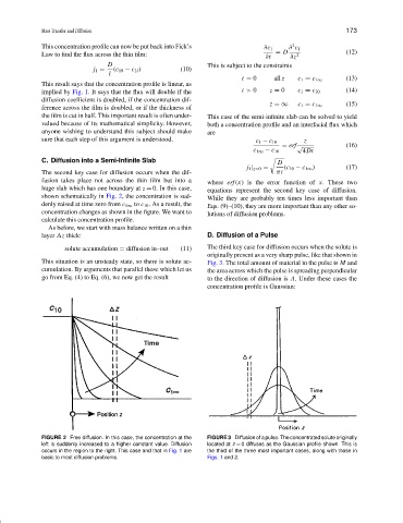
C. Diffusion into a Semi-Infinite Slab D
j 1 | z=0 = (c 10 − c 1∞ ) (17)
The second key case for diffusion occurs when the dif- πt
fusion takes place not across the thin film but into a where erf (x) is the error function of x. These two
huge slab which has one boundary at z = 0. In this case, equations represent the second key case of diffusion.
shown schematically in Fig. 2, the concentration is sud- While they are probably ten times less important than
denly raised at time zero from c 1∞ to c 10 . As a result, the Eqs. (9)–(10), they are more important than any other so-
concentration changes as shown in the figure. We want to lutions of diffusion problems.
calculate this concentration profile.
As before, we start with mass balance written on a thin
layer z thick: D. Diffusion of a Pulse

solute accumulation = diffusion in–out (11) The third key case for diffusion occurs when the solute is
originally present as a very sharp pulse, like that shown in
This situation is an unsteady state, so there is solute ac- Fig. 3. The total amount of material in the pulse is M and
cumulation. By arguments that parallel those which let us the area across which the pulse is spreading perpendicular
go from Eq. (4) to Eq. (6), we now get the result to the direction of diffusion is A. Under these cases the
concentration profile is Gaussian:

FIGURE 2 Free diffusion. In this case, the concentration at the FIGURE 3 Diffusion of a pulse. The concentrated solute originally
left is suddenly increased to a higher constant value. Diffusion located at z = 0 diffuses as the Gaussian profile shown. This is
occurs in the region to the right. This case and that in Fig. 1 are the third of the three most important cases, along with those in
basic to most diffusion problems. Figs. 1 and 2.