Page 323 - Academic Press Encyclopedia of Physical Science and Technology 3rd Analytical Chemistry

P1: GNH Final Pages
Encyclopedia of Physical Science and Technology EN009N-447 July 19, 2001 23:3

840 Microwave Molecular Spectroscopy

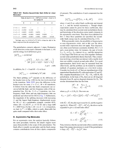
TABLE XXV Relative Second-Order Stark Shifts for Linear (if present). The contribution of each component has the
Molecules a form
2
Value of ∆[J(J + + 1) − − 3M ]/J(J + + 1)(2J − − 1)(2J + + 3) (2) 2 2 2
for various M E g Jτ M = µ A J,τ + B J,τ M , (111)
g
0 1 2 3 4 where A and B are called Stark coefficients and depend
on J, τ, and the inertial asymmetry κ. Though simple
J = 0 → 1 0.5333 — — — — expressions cannot be given for these coefficients, they
J = 1 → 2 −0.1524 0.1238 — — — may be calculated from second-order perturbation theory
J = 2 → 3 −0.0254 −0.0071 0.0476 — — and knowledge of the direction cosine matrix elements in
J = 3 → 4 −0.0092 −0.0056 0.0052 0.0288 — the asymmetric rotor basis. They have been tabulated for
J = 4 → 5 −0.0044 −0.0033 −0.0001 0.0054 0.0165 low J. Once these quantities are specified, the second-
order Stark energy may be calculated from Eq. (111).
a Multiply entry by (0.50344) µ /2B to obtain the shift of the
2 2 2
Stark component from the undisplaced line. With asymmetric rotors, the possibility of degeneracies
or near degeneracies exists, and in this case the above
second-order expression does not apply. Near degenera-
The perturbation connects adjacent J states. Evaluation cies often occur between asymmetry doublets. For J = 2
of the direction cosine matrix elements in the basis |J, M) and a near-prolate rotor, for instance, the pair of levels
and the energy level differences gives 2 1,2 ,2 1,1 or 2 2,1 ,2 2,0 interact via µ a , and this interaction

(2) 2 is very large if the levels are very close together. Ordinary
E = (0.50334)
J,M
second-order perturbation theory then fails. Thus a transi-
2
µ 2 " J(J + 1) − 3M 2 # tion involving a level that can interact with a nearby level
× , does not exhibit a typical second-order effect. To a good
2B J(J + 1)(2J − 1)(2J + 3)
approximation, these levels may be separated from the
J = 0 (109) other levels, and the problem can be treated by standard
methods of quantum mechanics as a two-level system.
In addition, for J = 0 and M = 0, we have 0 0
Consider two levels ψ , ψ that are eigenfunctions of the
2
1
0
0
(2) 2 2 2 unperturbed Hamiltonian 0 with eigenvalues E and E .
1
2
E J=0 =−(0.50344) µ /6B. (110) The complete Hamiltonian is = 0 + , with the
The Stark splitting ν (2) depends on the difference of perturbation. In the basis of 0 , there are no off-diagonal
elements from 0 and no diagonal elements for . The
the bracket term in Eq. (109) for the two levels involved
secular determinant thus has the form
in the transition. Table XXV gives the difference in the
bracket term for some J → J + 1, M → M transitions. E − E
0

1 µ 12
It follows from the table that Stark components can oc- 0 = 0, (112)
µ 12 E − E

2
cur on both the high- and low-frequency sides of the un-
perturbed line. For the J = 2 → 3 transition, two low- where µ 12 = (1| |2). The roots are
frequency Stark lobes and one high-frequency lobe are
1 0 0 1 0 0 2 2 2 1/2
predicted and observed for OCS in Fig. 3. Furthermore, E 1,2 = E + E ± E + E + 4 µ ,
2 1 2 2 1 2 12
the magnitude of the splitting decreases with increasing
(113)
J, and the largest high-frequency displacement occurs
for M = J. As a quantitative example, consider OCS, with E > E ; the plus sign is used for E 1 and the negative
0
0
1
2
where 2B = 12,162.97, µ = 0.715 D, and a large field sign for E 2 . When (E − E ) > 4 µ , the above can be
2
0 2
0
2
12
2
1
= 2800 V/cm. For the J, M = (2, 2) → (3, 2) transition, expanded to give a second-order effect:
we find ν (2) = 4 MHz, which is easily observable but
2
quite small compared with a first-order effect. 0 µ 2
12
E 1 = E + +· · · , (114)
1
0
E − E 0
1 2
B. Asymmetric-Top Molecules
2
µ 2
0 12
For an asymmetric rotor, the analysis basically follows E 2 = E − 0 0 +· · · . (115)
2
E − E 2
1
the same procedure; however, the details require more
space than possible in the scope of this presentation. The Note, however, that the second-order effect could be rather
Stark effect is usually second order, and the Stark energy large if the energy denominator is small. If the perturbation
2
2
0 2
0
contains contributions from all three dipole components is large, (E − E ) < 4µ , then
1 2 12