Page 142 - Engineering Electromagnetics, 8th Edition

124 ENGINEERING ELECTROMAGNETICS

5.5 THE METHOD OF IMAGES
One important characteristic of the dipole field that we developed in Chapter 4 is
the infinite plane at zero potential that exists midway between the two charges. Such
a plane may be represented by a vanishingly thin conducting plane that is infinite
in extent. The conductor is an equipotential surface at a potential V = 0, and the
electric field intensity is therefore normal to the surface. Thus, if we replace the
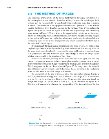
dipole configuration shown in Figure 5.6a with the single charge and conducting
plane shown in Figure 5.6b, the fields in the upper half of each figure are the same.
Below the conducting plane, all fields are zero, as we have not provided any charges
in that region. Of course, we might also substitute a single negative charge below a
conducting plane for the dipole arrangement and obtain equivalence for the fields in
the lower half of each region.
If we approach this equivalence from the opposite point of view, we begin with a
single charge above a perfectly conducting plane and then see that we may maintain
the same fields above the plane by removing the plane and locating a negative charge
at a symmetrical location below the plane. This charge is called the image of the
original charge, and it is the negative of that value.
If we can do this once, linearity allows us to do it again and again, and thus any
charge configuration above an infinite ground plane may be replaced by an arrange-
ment composed of the given charge configuration, its image, and no conducting plane.
This is suggested by the two illustrations of Figure 5.7. In many cases, the potential
field of the new system is much easier to find since it does not contain the conducting
plane with its unknown surface charge distribution.
As an example of the use of images, let us find the surface charge density at
P(2, 5, 0) on the conducting plane z = 0if there is a line charge of 30 nC/m located
at x = 0, z = 3, as shown in Figure 5.8a.We remove the plane and install an
image line charge of −30 nC/m at x = 0, z =−3, as illustrated in Figure 5.8b.
The field at P may now be obtained by superposition of the known fields of the line

Figure 5.6 (a)Two equal but opposite charges may be replaced by (b)a single charge
and a conducting plane without affecting the fields above the V = 0 surface.