Page 213 - Engineering Electromagnetics, 8th Edition

CHAPTER 7 The Steady Magnetic Field 195

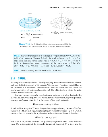
Figure 7.12 (a)An ideal toroid carrying a surface current K in the
direction shown. (b)An N-turn toroid carrying a filamentary current I.

D7.3. Express the value of H in rectangular components at P(0, 0.2, 0) in the
field of: (a)a current filament, 2.5 A in the a z direction at x = 0.1, y = 0.3;
(b)a coax, centered on the z axis, with a = 0.3, b = 0.5, c = 0.6, I = 2.5A
in the a z direction in the center conductor; (c) three current sheets, 2.7a x A/m
at y = 0.1, −1.4a x A/m at y = 0.15, and −1.3a x A/m at y = 0.25.

Ans. 1.989a x − 1.989a y A/m; −0.884a x A/m; 1.300a z A/m

7.3 CURL
We completed our study of Gauss’s law by applying it to a differential volume element
and were led to the concept of divergence. We now apply Amp`ere’s circuital law to
the perimeter of a differential surface element and discuss the third and last of the
special derivatives of vector analysis, the curl. Our objective is to obtain the point
form of Amp`ere’s circuital law.
Again we choose rectangular coordinates, and an incremental closed path of sides
x and y is selected (Figure 7.13). We assume that some current, as yet unspecified,
produces a reference value for H at the center of this small rectangle,

H 0 = H x0 a x + H y0 a y + H z0 a z
The closed line integral of H about this path is then approximately the sum of the four
values of H · L on each side. We choose the direction of traverse as 1-2-3-4-1, which
corresponds to a current in the a z direction, and the first contribution is therefore

(H · L) 1−2 = H y,1−2 y
The value of H y on this section of the path may be given in terms of the reference
value H y0 at the center of the rectangle, the rate of change of H y with x, and the