Page 299 - Engineering Electromagnetics, 8th Edition

CHAPTER 9 Time-Varying Fields and Maxwell’s Equations 281

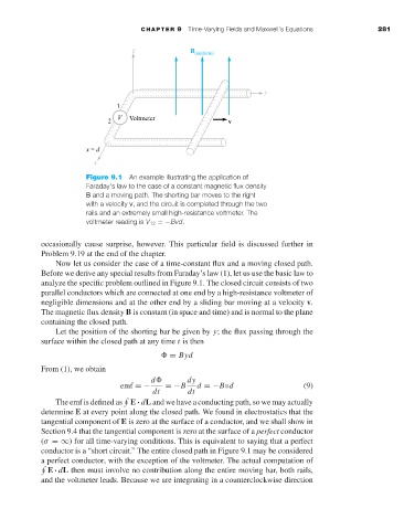
Figure 9.1 An example illustrating the application of
Faraday’s law to the case of a constant magnetic flux density
B and a moving path. The shorting bar moves to the right
with a velocity v, and the circuit is completed through the two
rails and an extremely small high-resistance voltmeter. The
voltmeter reading is V 12 =−Bvd.

occasionally cause surprise, however. This particular field is discussed further in
Problem 9.19 at the end of the chapter.
Now let us consider the case of a time-constant flux and a moving closed path.
Before we derive any special results from Faraday’s law (1), let us use the basic law to
analyze the specific problem outlined in Figure 9.1. The closed circuit consists of two
parallel conductors which are connected at one end by a high-resistance voltmeter of
negligible dimensions and at the other end by a sliding bar moving at a velocity v.
The magnetic flux density B is constant (in space and time) and is normal to the plane
containing the closed path.
Let the position of the shorting bar be given by y; the flux passing through the
surface within the closed path at any time t is then

= Byd
From (1), we obtain
d dy
emf =− =−B d =−Bνd (9)
dt dt
The emf is defined as E · dL and we have a conducting path, so we may actually

determine E at every point along the closed path. We found in electrostatics that the
tangential component of E is zero at the surface of a conductor, and we shall show in
Section 9.4 that the tangential component is zero at the surface of a perfect conductor
(σ =∞) for all time-varying conditions. This is equivalent to saying that a perfect
conductor is a “short circuit.” The entire closed path in Figure 9.1 may be considered
a perfect conductor, with the exception of the voltmeter. The actual computation of
E · dL then must involve no contribution along the entire moving bar, both rails,

and the voltmeter leads. Because we are integrating in a counterclockwise direction