Page 301 - Engineering Electromagnetics, 8th Edition

CHAPTER 9 Time-Varying Fields and Maxwell’s Equations 283

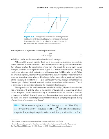
Figure 9.2 An apparent increase in flux linkages does
not lead to an induced voltage when one part of a circuit
is simply substituted for another by opening the switch.
No indication will be observed on the voltmeter.

This expression is equivalent to the simple statement

d
emf =− (1)
dt
and either can be used to determine these induced voltages.
Although (1) appears simple, there are a few contrived examples in which its
proper application is quite difficult. These usually involve sliding contacts or switches;
4
they always involve the substitution of one part of a circuit by a new part. As an
example, consider the simple circuit of Figure 9.2, which contains several perfectly
conducting wires, an ideal voltmeter, a uniform constant field B, and a switch. When
the switch is opened, there is obviously more flux enclosed in the voltmeter circuit;
however, it continues to read zero. The change in flux has not been produced by either
a time-changing B [first term of (14)] or a conductor moving through a magnetic field
[second part of (14)]. Instead, a new circuit has been substituted for the old. Thus it
is necessary to use care in evaluating the change in flux linkages.
The separation of the emf into the two parts indicated by (14), one due to the time
rate of change of B and the other to the motion of the circuit, is somewhat arbitrary
in that it depends on the relative velocity of the observer and the system. A field that
is changing with both time and space may look constant to an observer moving with
the field. This line of reasoning is developed more fully in applying the special theory
of relativity to electromagnetic theory. 5

D9.1. Within a certain region, = 10 −11 F/m and µ = 10 −5 H/m. If B x =
∂E
5
2×10 −4 cos 10 t sin 10 −3 y T: (a) use ∇×H = to find E;(b) find the total
∂t
magnetic flux passing through the surface x = 0, 0 < y < 40 m, 0 < z < 2m,

4 See Bewley, in References at the end of the chapter, particularly pp. 12–19.
5 This is discussed in several of the references listed in the References at the end of the chapter.
See Panofsky and Phillips, pp. 142–51; Owen, pp. 231–45; and Harman in several places.