Page 323 - Engineering Electromagnetics, 8th Edition

CHAPTER 10 Transmission Lines 305

KCL +

g
c
+

KVL

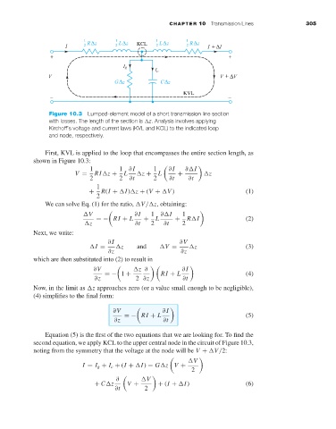
Figure 10.3 Lumped-element model of a short transmission line section
with losses. The length of the section is z. Analysis involves applying
Kirchoff’s voltage and current laws (KVL and KCL) to the indicated loop
and node, respectively.

First, KVL is applied to the loop that encompasses the entire section length, as
shown in Figure 10.3:
1 1 ∂ I 1 ∂ I ∂ I
V = RI z + L z + L + z
2 2 ∂t 2 ∂t ∂t
1
+ R(I + I) z + (V + V ) (1)
2
We can solve Eq. (1) for the ratio, V/ z, obtaining:
V =− RI + L ∂ I 1 ∂ I 1 R I (2)

L
z ∂t + 2 ∂t + 2
Next, we write:
∂ I ∂V
I = z and V = z (3)
∂z ∂z
which are then substituted into (2) to result in
∂V z ∂ ∂ I
=− 1 + RI + L (4)
∂z 2 ∂z ∂t
Now, in the limit as z approaches zero (or a value small enough to be negligible),
(4) simplifies to the final form:

∂V =− RI + L ∂ I (5)

∂z ∂t
Equation (5) is the first of the two equations that we are looking for. To find the
second equation, we apply KCL to the upper central node in the circuit of Figure 10.3,
noting from the symmetry that the voltage at the node will be V + V/2:
V

I = I g + I c + (I + I) = G z V +
2

∂ V
+ C z V + + (I + I) (6)
∂t 2