Page 530 - Engineering Electromagnetics, 8th Edition

512 ENGINEERING ELECTROMAGNETICS

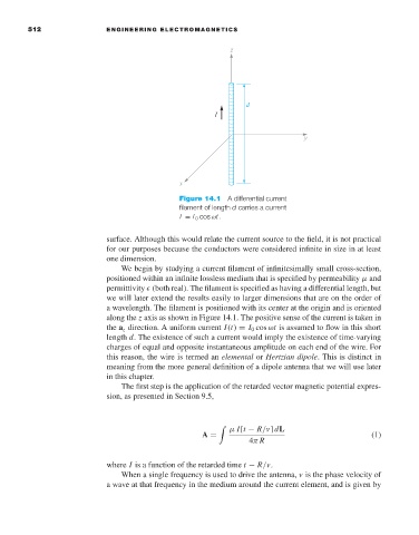
Figure 14.1 A differential current
filament of length d carries a current
I = I 0 cos ωt.

surface. Although this would relate the current source to the field, it is not practical
for our purposes because the conductors were considered infinite in size in at least
one dimension.
We begin by studying a current filament of infinitesimally small cross-section,
positioned within an infinite lossless medium that is specified by permeability µ and
permittivity (both real). The filament is specified as having a differential length, but
we will later extend the results easily to larger dimensions that are on the order of
awavelength. The filament is positioned with its center at the origin and is oriented
along the z axis as shown in Figure 14.1. The positive sense of the current is taken in
the a z direction. A uniform current I(t) = I 0 cos ωt is assumed to flow in this short
length d. The existence of such a current would imply the existence of time-varying
charges of equal and opposite instantaneous amplitude on each end of the wire. For
this reason, the wire is termed an elemental or Hertzian dipole. This is distinct in
meaning from the more general definition of a dipole antenna that we will use later
in this chapter.
The first step is the application of the retarded vector magnetic potential expres-
sion, as presented in Section 9.5,

µ I[t − R/v] dL

A = (1)
4π R

where I is a function of the retarded time t − R/v.
When a single frequency is used to drive the antenna, v is the phase velocity of
awaveat that frequency in the medium around the current element, and is given by