Page 141 - Essentials of applied mathematics for scientists and engineers

book Mobk070 March 22, 2007 11:7

SOLUTIONS WITH LAPLACE TRANSFORMS 131
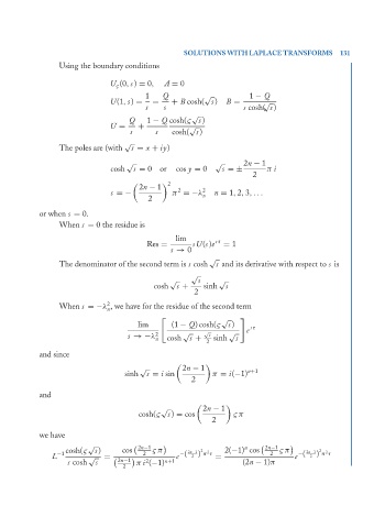
Using the boundary conditions

U ς (0, s ) = 0, A = 0
1 Q √ 1 − Q
U(1, s ) = = + B cosh( s ) B = √
s s s cosh( s )
√
Q 1 − Q cosh(ς s )
U = + √
s s cosh( s )
√
The poles are (with s = x + iy)
√ √ 2n − 1
cosh s = 0or cos y = 0 s =± π i
2
2
2n − 1

2
s =− π =−λ 2 n n = 1, 2, 3,...
2
or when s = 0.
When s = 0 the residue is

lim s τ
Res = sU(s )e = 1
s → 0
√
The denominator of the second term is s cosh s and its derivative with respect to s is
√
√ s √
cosh s + sinh s
2
2
When s =−λ ,wehavefor theresidue of thesecondterm
n
√
lim (1 − Q)cosh(ς s ) s τ
s →−λ 2 √ √ s √ e
n cosh s + sinh s
2
and since

√ 2n − 1
sinh s = i sin π = i(−1) n+1
2
and

√ 2n − 1
cosh(ς s ) = cos ςπ
2
we have
√ 2n−1 n 2n−1
cosh(ς s ) cos ςπ 2n−1 2 2 2(−1) cos ςπ 2n−1 2 2
L −1 √ = 2 e −( 2 ) π τ = 2 e −( 2 ) π τ
s cosh s 2n−1 π i (−1) n+1 (2n − 1)π
2
2