Page 121 - Essentials of physical chemistry

The Second and Third Laws of Thermodynamics 83

Cancel

Survive

Pressure, P

Volume, V
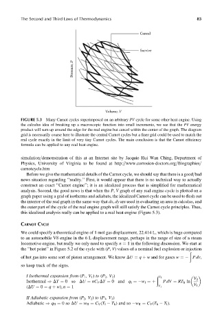
FIGURE 5.3 Many Carnot cycles superimposed on an arbitrary PV cycle for some other heat engine. Using
the calculus idea of breaking up a macroscopic function into small increments, we see that the PV energy
product will sum up around the edge for the real engine but cancel within the center of the graph. The diagram
grid is necessarily coarse here to illustrate the central Carnot cycles but a finer grid could be used to match the
real cycle exactly in the limit of very tiny Carnot cycles. The main conclusion is that the Carnot efficiency
formula can be applied to any real heat engine.

simulation=demonstration of this at an Internet site by Jacquie Hui Wan Ching, Department of
Physics, University of Virginia to be found at http:==www.corrosion-doctors.org=Biographies=
carnotcycle.htm
Before we give the mathematical details of the Carnot cycle, we should say that there is a good=bad
news situation regarding ‘‘reality.’’ First, it would appear that there is no technical way to actually
construct an exact ‘‘Carnot engine’’; it is an idealized process that is simplified for mathematical
analysis. Second, the good news is that when the P, V graph of any real engine cycle is plotted on a
graph paper using a grid of isotherms and adiabats, the idealized Carnot cycle can be used to flesh out
the interior of the real graph in the same way that dx, dy are used in evaluating an area in calculus, and
the outer part of the cycle of the real engine graph will still satisfy the Carnot cycle principles. Thus,
this idealized analysis really can be applied to a real heat engine (Figure 5.3).

CARNOT CYCLE
We could specify a theoretical engine of 1 mol gas displacement, 22.414 L, which is huge compared
to an automobile V8 engine in the 6 L displacement range, perhaps in the range of size of a steam
locomotive engine, but really we only need to specify n ¼ 1 in the following discussion. We start at
the ‘‘hot point’’ in Figure 5.2 of the cycle with (P, V) values of a nominal fuel explosion or injection
ð
of hot gas into some sort of piston arrangement. We know DU ¼ q þ w and for gases w ¼ Pdv,
so keep track of the signs.

I Isothermal expansion from (P 1 ,V 1 ) to (P 2 ,V 2 ) ð V 2
V 2
PdV ¼ RT h ln
Isothermal ) DT ¼ 0so DU ¼ nC V DT ¼ 0 and q I ¼ w I ¼þ
(DU ¼ 0 ¼ q þ w), n ¼ 1 V 1 V 1
II Adiabatic expansion from (P 2 ,V 2 ) to (P 3 ,V 3 )
Adiabatic ) q II ¼ 0so DU ¼ w II ¼ C V (T l T h ) and so w II ¼ C V (T h T l ).