Page 122 - Essentials of physical chemistry

84 Essentials of Physical Chemistry

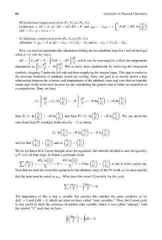
III Isothermal compression from (P 3 ,V 3 ) to (P 4 ,V 4 ) ð
V 4
V 4
PdV ¼ RT l ln
Isothermal ) DT ¼ 0so DU ¼ nC V DT ¼ 0 and q III ¼ w III ¼þ
V 3
(DU ¼ 0 ¼ q þ w), n ¼ 1. V 3
IV Adiabatic compression from (P 4 ,V 4 ) to (P 1 ,V 1 )
Adiabatic ) q IV ¼ 0so DU ¼ w IV ¼ C V (T h T l ) and so w IV ¼ C V (T l T h ).

Now, we need an important side calculation relating the two adiabatic steps for 1 mol of ideal gas
when q ¼ 0. (the key step.)
dV
ð ð ð
DU ¼ C V dT ¼ 0 PdV ¼ RT , which can be rearranged to collect the temperature
dT dV
ð ð V
dependence as C V ¼ R . This is easily done algebraically by removing the integration
T V
symbols, dragging T under the left side and then reapplying the integral signs. This step is similar to
the previous treatment of adiabatic nozzle jet cooling. Here, our goal is to merely derive a key
relationship between the volumes and temperatures of the adiabatic steps and note that we kept the
minus sign on the work term because we are considering the general case of either an expansion or
a compression. Thus, we have

T ð 2 V ð 2
dT T 2 dV V 2 V 1
C V ¼ C V ln ¼ R ¼ R ln ¼þR ln :
T T 1 V V 1 V 2
T 1 V 1

T l V 3 T h V 1
Step II: C V ln ¼ R ln and Step IV: C V ln ¼ R ln . We can invert the
T h V 2 T l V 4
ratio from Step IV (multiply both sides by 1) to obtain

T l V 4 V 3
C V ln ¼ R ln ¼ R ln
T h V 1 V 2

V 4 V 3 V 4 V 1
and we find ¼ and so ¼ .
V 1 V 2 V 3 V 2
We do not know how Carnot thought about the equations, but when he decided to sum the quantity,
q=T, over all four steps, he found a profound result.

RT h ln V 2 RT l ln V 4
X
q rev V 1 V 3 V 4 V 1
þ 0 but ¼ so the ln terms cancel out.
þ 0 þ
¼
T T h T l V 3 V 2
Note that we used the reversible equation for the adiabatic steps of the PV work, so we must specify
that the heat term be noted as q rev . What does this mean? Concisely for the cycle
þ
X
q rev dq rev
¼ 0:
T ¼ T
The importance of this is that a variable that satisfies this matches the same condition as for
Þ Þ
dU ¼ 0and dH ¼ 0, which are what we have called ‘‘state variables.’’ Thus, the Carnot cycle
is very useful to show the existence of another state variable, which is now called ‘‘entropy’’ with
the symbol ‘‘S’’ such that we have

þ þ
dq rev
¼ dS ¼ 0:
T