Page 319 - Excel 2007 Bible

20_044039 ch15.qxp 11/21/06 11:07 AM Page 276
Part II
Working with Formulas and Functions
The VLOOKUP function
The VLOOKUP function looks up the value in the first column of the lookup table and returns the corre-
sponding value in a specified table column. The lookup table is arranged vertically (which explains the
V in the function’s name). The syntax for the VLOOKUP function is
VLOOKUP(lookup_value,table_array,col_index_num,range_lookup)
The VLOOKUP function’s arguments are as follows:
n lookup_value: The value to be looked up in the first column of the lookup table.
n table_array: The range that contains the lookup table.
n col_index_num: The column number within the table from which the matching value is returned.
n range_lookup: Optional. If TRUE or omitted, an approximate match is returned. (If an exact
match is not found, the next largest value that is less than lookup_value is returned.) If FALSE,
VLOOKUP will search for an exact match. If VLOOKUP can’t find an exact match, the function
returns #N/A.
If the range_lookup argument is TRUE or omitted, the first column of the lookup table must
NOTE
NOTE
be in ascending order. If lookup_value is smaller than the smallest value in the first column of
table_array, VLOOKUP returns #N/A. If the range_lookup argument is FALSE, the first column of the lookup
table need not be in ascending order. If an exact match is not found, the function returns #N/A.
TIP If the lookup_value argument is text, it can include wildcard characters * and ?.
TIP
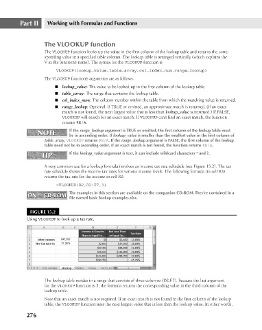
A very common use for a lookup formula involves an income tax rate schedule (see Figure 15.2). The tax
rate schedule shows the income tax rates for various income levels. The following formula (in cell B3)
returns the tax rate for the income in cell B2:
=VLOOKUP(B2,D2:F7,3)
The examples in this section are available on the companion CD-ROM. They’re contained in a
ON the CD-ROM
ON the CD-ROM file named basic lookup examples.xlsx.
FIGURE 15.2
Using VLOOKUP to look up a tax rate.
The lookup table resides in a range that consists of three columns (D2:F7). Because the last argument
for the VLOOKUP function is 3, the formula returns the corresponding value in the third column of the
lookup table.
Note that an exact match is not required. If an exact match is not found in the first column of the lookup
table, the VLOOKUP function uses the next largest value that is less than the lookup value. In other words,

276