Page 324 - Excel 2007 Bible

20_044039 ch15.qxp 11/21/06 11:07 AM Page 281
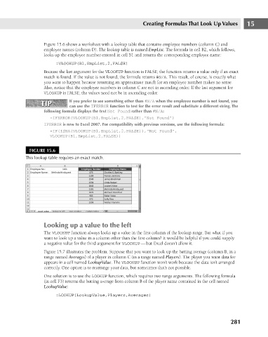
Figure 15.6 shows a worksheet with a lookup table that contains employee numbers (column C) and
employee names (column D). The lookup table is named EmpList. The formula in cell B2, which follows,
looks up the employee number entered in cell B1 and returns the corresponding employee name:
Because the last argument for the VLOOKUP function is FALSE, the function returns a value only if an exact
match is found. If the value is not found, the formula returns #N/A. This result, of course, is exactly what
you want to happen because returning an approximate match for an employee number makes no sense.
Also, notice that the employee numbers in column C are not in ascending order. If the last argument for
VLOOKUP is FALSE, the values need not be in ascending order.
If you prefer to see something other than #N/A when the employee number is not found, you
TIP
TIP
can use the IFERROR function to test for the error result and substitute a different string. The
following formula displays the text Not Found rather than #N/A:
=IFERROR(VLOOKUP(B1,EmpList,2,FALSE),”Not Found”)
IFERROR is new to Excel 2007. For compatibility with previous versions, use the following formula:
=IF(ISNA(VLOOKUP(B1,EmpList,2,FALSE)),”Not Found”,
VLOOKUP(B1,EmpList,2,FALSE))
FIGURE 15.6 =VLOOKUP(B1,EmpList,2,FALSE) Creating Formulas That Look Up Values 15
This lookup table requires an exact match.
Looking up a value to the left
The VLOOKUP function always looks up a value in the first column of the lookup range. But what if you
want to look up a value in a column other than the first column? It would be helpful if you could supply
a negative value for the third argument for VLOOKUP — but Excel doesn’t allow it.
Figure 15.7 illustrates the problem. Suppose that you want to look up the batting average (column B, in a
range named Averages) of a player in column C (in a range named Players). The player you want data for
appears in a cell named LookupValue. The VLOOKUP function won’t work because the data isn’t arranged
correctly. One option is to rearrange your data, but sometimes that’s not possible.
One solution is to use the LOOKUP function, which requires two range arguments. The following formula
(in cell F3) returns the batting average from column B of the player name contained in the cell named
LookupValue:
=LOOKUP(LookupValue,Players,Averages)

281