Page 327 - Excel 2007 Bible

20_044039 ch15.qxp 11/21/06 11:07 AM Page 284
Part II
Working with Formulas and Functions
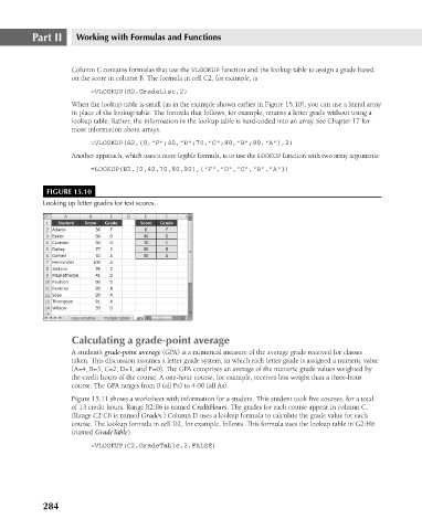
Column C contains formulas that use the VLOOKUP function and the lookup table to assign a grade based
on the score in column B. The formula in cell C2, for example, is
=VLOOKUP(B2,GradeList,2)
When the lookup table is small (as in the example shown earlier in Figure 15.10), you can use a literal array
in place of the lookup table. The formula that follows, for example, returns a letter grade without using a
lookup table. Rather, the information in the lookup table is hard-coded into an array. See Chapter 17 for
more information about arrays.
=VLOOKUP(B2,{0,”F”;40,”D”;70,”C”;80,”B”;90,”A”},2)
Another approach, which uses a more legible formula, is to use the LOOKUP function with two array arguments:
=LOOKUP(B2,{0,40,70,80,90},{“F”,”D”,”C”,”B”,”A”})
FIGURE 15.10
Looking up letter grades for test scores.

Calculating a grade-point average
A student’s grade-point average (GPA) is a numerical measure of the average grade received for classes
taken. This discussion assumes a letter grade system, in which each letter grade is assigned a numeric value
(A=4, B=3, C=2, D=1, and F=0). The GPA comprises an average of the numeric grade values weighted by
the credit hours of the course. A one-hour course, for example, receives less weight than a three-hour
course. The GPA ranges from 0 (all Fs) to 4.00 (all As).
Figure 15.11 shows a worksheet with information for a student. This student took five courses, for a total
of 13 credit hours. Range B2:B6 is named CreditHours. The grades for each course appear in column C.
(Range C2:C6 is named Grades.) Column D uses a lookup formula to calculate the grade value for each
course. The lookup formula in cell D2, for example, follows. This formula uses the lookup table in G2:H6
(named GradeTable).

=VLOOKUP(C2,GradeTable,2,FALSE)

284