Page 329 - Excel 2007 Bible

20_044039 ch15.qxp 11/21/06 11:07 AM Page 286
Part II
Working with Formulas and Functions
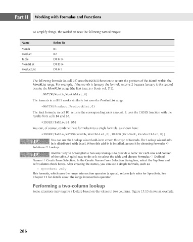
To simplify things, the worksheet uses the following named ranges:
Refers To
Name
B1
Month
B2
Product
Table
D1:H14
D1:D14
MonthList
D1:H1
ProductList
The following formula (in cell B4) uses the MATCH function to return the position of the Month within the
MonthList range. For example, if the month is January, the formula returns 2 because January is the second
item in the MonthList range (the first item is a blank cell, D1).
=MATCH(Month,MonthList,0)
The formula in cell B5 works similarly but uses the ProductList range.
=MATCH(Product,ProductList,0)
The final formula, in cell B6, returns the corresponding sales amount. It uses the INDEX function with the
results from cells B4 and B5.
=INDEX(Table,B4,B5)
You can, of course, combine these formulas into a single formula, as shown here:
=INDEX(Table,MATCH(Month,MonthList,0),MATCH(Product,ProductList,0))
TIP You can use the Lookup wizard add-in to create this type of formula. The Lookup wizard add-
TIP
in is distributed with Excel. When this add-in is installed, access it by choosing Formulas ➪
Solutions ➪ Lookup.
TIP Another way to accomplish a two-way lookup is to provide a name for each row and column
TIP
of the table. A quick way to do so is to select the table and choose Formulas ➪ Defined
Names ➪ Create From Selection. In the Create Names From Selection dialog box, select the Top Row and
Left Column check boxes. After creating the names, you can use a simple formula, such as:
= Sprockets July
This formula, which uses the range intersection operator (a space), returns July sales for Sprockets. See
Chapter 11 for details about the range intersection operator.
Performing a two-column lookup
Some situations may require a lookup based on the values in two columns. Figure 15.13 shows an example.

286