Page 331 - Excel 2007 Bible

20_044039 ch15.qxp 11/21/06 11:07 AM Page 288
Part II
Working with Formulas and Functions
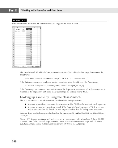
FIGURE 15.14
The formula in cell B2 returns the address in the Data range for the value in cell B1.
The formula in cell B2, which follows, returns the address of the cell in the Data range that contains the
Target value:
=ADDRESS(ROW(Data)+MATCH(Target,Data,0)-1,COLUMN(Data))
If the Data range occupies a single row, use this formula to return the address of the Target value:
=ADDRESS(ROW(Data),COLUMN(Data)+MATCH(Target,Data,0)-1)
If the Data range contains more than one instance of the Target value, the address of the first occurrence is
returned. If the Target value isn’t found in the Data range, the formula returns #N/A.

Looking up a value by using the closest match
The VLOOKUP and HLOOKUP functions are useful in the following situations:
n You need to identify an exact match for a target value. Use FALSE as the function’s fourth argument.
n You need to locate an approximate match. If the function’s fourth argument is TRUE or omitted
and an exact match is not found, the next largest value less than the lookup value is returned.
But what if you need to look up a value based on the closest match? Neither VLOOKUP nor HLOOKUP can
do the job.
Figure 15.15 shows a worksheet with student names in column A and values in column B. Range B2:B20
is named Data. Cell E2, named Target, contains a value to search for in the Data range. Cell E3, named
ColOffset, contains a value that represents the column offset from the Data range.

288