Page 91 - Excel Data Analysis

05 537547 Ch04.qxd 3/4/03 11:52 AM Page 77

CREATING FORMULAS 4

You can combine the results of the MATCH function with To find the location of specific text
other functions to locate related values within a data list. within a worksheet row or column, you
For example, you can use the row value that the MATCH use the wildcard characters of an
function returns to determine which month had the highest asterisk, *, to match multiple characters
sales figures under $400,000. To do this most effectively, you or a question mark, ?, to match a single
combine the MATCH function with the INDEX function. The character. With these characters, you
following formula has the MATCH function representing the must specify a value of 0 for the
Row_num argument of the INDEX function. See the section match_type argument.
"Return a Value at a Specific Location in a Data List" for TYPE THIS:
more information on the INDEX function.

=MATCH(ch*t, A1:A25, 0)
TYPE THIS:
=INDEX(A1:C49,(MATCH(400000,C1:C49,1)),1)
RESULT:

RESULT: Excel finds the first value in the cell
range that starts with "ch" and ends
with "t".
The INDEX function returns a cell value from the data
list range A1:C49. The MATCH function locates the row
value, and 1 specifies the column number, which in this
case is Column A.

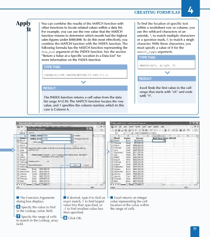
■ The Function Arguments ■ If desired, type 0 to find an ■ Excel returns an integer
dialog box displays. exact match, 1 to find largest value representing the cell
value less than specified, or location of the value within
Á Specify the value to find -1 to find smallest value less the range of cells.
in the Lookup_value field.
than specified.
‡ Specify the range of cells ° Click OK.
to search in the Lookup_array
field.
77