Page 93 - Excel Data Analysis

05 537547 Ch04.qxd 3/4/03 11:52 AM Page 79

CREATING FORMULAS 4

To quickly find a value in a data list when you do not want to
manually create a formula, you can use the Lookup Wizard option
which allows you to find a value based upon the row and column
labels. By selecting a particular row and column heading, Excel
creates a formula that returns the intersection. The Lookup Wizard is
available as part of the Add-Ins that come with Excel. See Chapter 11
for more information.
After you load the Lookup Wizard Add-in, you can click Tools ➪
Lookup to run it. The Lookup Wizard consists of four different steps,
or pages. On the first page, you specify the range of cells you want
to search. On the second page you select the appropriate column
and row labels. This Wizard works best if you have unique row and
column labels. If you have duplicate row or column labels, the
Wizard may return the wrong value.
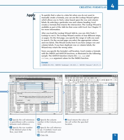
Next, you specify the formula's cell location. Excel creates a formula
with the INDEX and MATCH functions, as illustrated in the following
sample. The MATCH function returns the row_num and
column_num argument values for the INDEX function.
Example:
=INDEX(B1:F20, MATCH("Andrews",B1:B20,), MATCH("Amount",B1:F1,))

Á Specify the cell references ° Specify the column ■ Excel returns the value of
in parentheses with a comma number in the Column_num the cell within the specified
between each reference. field. location.
‡ Specify the row number · Specify the cell reference
of the desired value in the to use. If omitted, Excel uses
Row_num field. the first cell reference.
‚ Click OK. 79