Page 181 - Excel Timesaving Techniques for Dummies

34_574272 ch30.qxd 10/1/04 10:50 PM Page 166
166
Technique 30: Creating Efficient Date and Time Formulas
The only problem, as you can see in Figure 30-2, is
that the program applies the most common Date
number format to the calculated results so that the
difference in cell G2 appears as the date

9/10/1916
To display the results in column G as whole num-
bers, as you’d expect, you have to then format the
calculated differences with another number format.
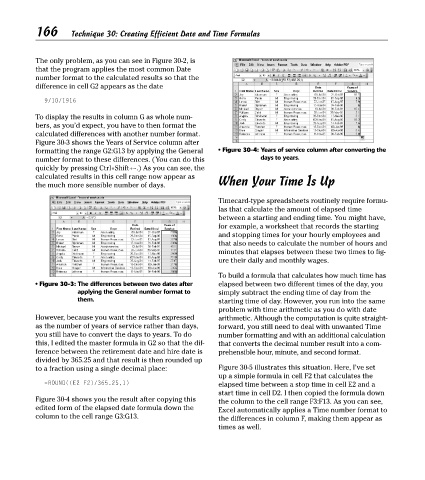
Figure 30-3 shows the Years of Service column after
formatting the range G2:G13 by applying the General • Figure 30-4: Years of service column after converting the
number format to these differences. (You can do this days to years.
quickly by pressing Ctrl+Shift+~.) As you can see, the
calculated results in this cell range now appear as When Your Time Is Up
the much more sensible number of days.

Timecard-type spreadsheets routinely require formu-
las that calculate the amount of elapsed time
between a starting and ending time. You might have,
for example, a worksheet that records the starting
and stopping times for your hourly employees and
that also needs to calculate the number of hours and
minutes that elapses between these two times to fig-
ure their daily and monthly wages.
To build a formula that calculates how much time has
• Figure 30-3: The differences between two dates after elapsed between two different times of the day, you
applying the General number format to simply subtract the ending time of day from the
them. starting time of day. However, you run into the same
problem with time arithmetic as you do with date
However, because you want the results expressed arithmetic. Although the computation is quite straight-
as the number of years of service rather than days, forward, you still need to deal with unwanted Time
you still have to convert the days to years. To do number formatting and with an additional calculation
this, I edited the master formula in G2 so that the dif- that converts the decimal number result into a com-
ference between the retirement date and hire date is prehensible hour, minute, and second format.
divided by 365.25 and that result is then rounded up
to a fraction using a single decimal place: Figure 30-5 illustrates this situation. Here, I’ve set
up a simple formula in cell F2 that calculates the
=ROUND((E2-F2)/365.25,1) elapsed time between a stop time in cell E2 and a
start time in cell D2. I then copied the formula down
Figure 30-4 shows you the result after copying this the column to the cell range F3:F13. As you can see,
edited form of the elapsed date formula down the Excel automatically applies a Time number format to
column to the cell range G3:G13. the differences in column F, making them appear as
times as well.