Page 254 - Excel Workbook for Dummies

26_798452 ch18.qxp 3/13/06 7:45 PM Page 237
Chapter 18: Performing What-If Analysis 237

Be sure to select cell C7 and D7 as a range with the cell cursor before you drag
the Fill handle across the row to cell G7.
9. Select the data table’s cell range B7:G18 and then choose the Data➪Table
command.
10. Select the Expense_Rate cell, B4, as the Row Input Cell and the Growth_Rate cell,
B3, as the Column Input Cell in the Table dialog box. Select OK.
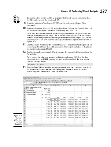
Excel then fills in the data table, substituting in succession the growth rate per-
centage entered in the cell range C8:C18 for the Growth_Rate cell in the master
formula and the expense rate percentage entered in the cell range C7:G7 for the
Expense_Rate cell. Check your results in your data table against those shown in
Figure 18-2.

11. Use the Format Painter on the Standard toolbar to copy the formatting in cell C8
to the range C8:G18 and then widen columns D through G sufficient to display all
the entries in the range D8:G18.
12. Position the cell cursor in cell C8 and examine the contents of the formula on the
Formula bar.
Excel inserts the following array formula in the cell range C8:G18 of the data
table (note that the TABLE function in this formula uses both the row_ref and
column_ref arguments):
={TABLE(B4,B3)}
13. Save the Data Table worksheet with your two-variable data table in a new work-
book with the filename Solved18-2.xls in your Chapter 18 folder in the My
Practice Spreadsheets folder. Close the workbook.

Figure 18-2:
The com-
pleted two-
variable
data table.