Page 102 - Excel for Scientists and Engineers: Numerical Methods

CHAPTER 5 INTERPOLATION 79

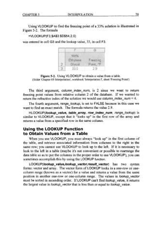
Using VLOOKUP to find the freezing point of a 33% solution is illustrated in
Figure 5-2. The formula
=VLOOKUP(F3,$A$3:$D$54,2,0)

was entered in cell G3 and the lookup value, 33, in cell F3.

Figure 5-2. Using VLOOKUP to obtain a value from a table.
(folder 'Chapter 05 Interpolation', workbook 'Interpolation I', sheet 'Freezing Point')

The third argument, column-index-num, is 2 since we want to return
freezing point values from relative column 2 of the database. If we wanted to
return the refractive index of the solution we would use column-index-num = 4.
The fourth argument, range-lookup, is set to FALSE because in this case we
want to find an exact match. The formula returns the value 2.9.
HLOOKU P(/ookup-value, table-array, row-index-num, range-lookup) is
similar to VLOOKUP, except that it "looks up" in the first row of the array and
returns a value from a specified row in the same column.

Using the LOOKUP Function
to Obtain Values from a Table
When you use VLOOKUP, you must always "look up" in the first column of
the table, and retrieve associated information from columns to the right in the
same row; you cannot use VLOOKUP to look up to the left. If it is necessary to
look to the left in a table (maybe it's not convenient or possible to rearrange the
data table so as to put the columns in the proper order to use VLOOKUP), you can
sometimes accomplish this by using the LOOKUP function.
LOOKUP(/ookup-va/ue,/ookup-vector,resu/t-vecfor) has two syntax
forms: vector and array. The vector form of LOOKUP looks in a one-row or one-
column range (known as a vector) for a value and returns a value from the same
position in another one-row or one-column range. The values in lookup-vector
must be sorted in ascending order. If LOOKUP can't find lookup-value, it returns
the largest value in lookup-vector that is less than or equal to lookup-value.