Page 103 - Excel for Scientists and Engineers: Numerical Methods

80 EXCEL: NUMERICAL METHODS

Creating a Custom Lookup Formula
to Obtain Values from a Table

A second way to "lookup" to the left in a table is to construct your own
lookup formula using Excel's MATCH and INDEX worksheet functions. The
MATCH and INDEX functions are almost mirror images of one another: MATCH
looks up a value in an array and returns its numerical position, INDEX looks in an
array and returns a value from a specified numerical position.
The following example illustrates how to use INDEX and MATCH to lookup
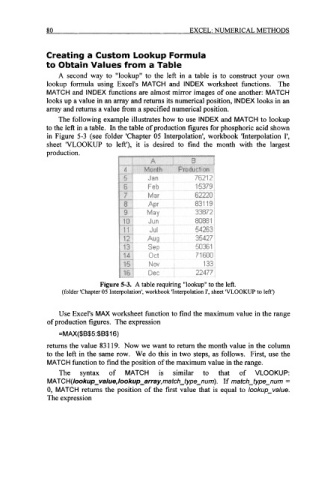
to the left in a table. In the table of production figures for phosphoric acid shown
in Figure 5-3 (see folder 'Chapter 05 Interpolation', workbook 'Interpolation 1',
sheet 'VLOOKUP to left'), it is desired to find the month with the largest
production.

Figure 5-3. A table requiring "lookup" to the left.
(folder 'Chapter 05 Interpolation', workbook 'Interpolation I', sheet 'VLOOKUP to left')

Use Excel's MAX worksheet function to find the maximum value in the range
of production figures. The expression
=MAX($B$S:$B$lG)
returns the value 83 1 19. Now we want to return the month value in the column
to the left in the same row. We do this in two steps, as follows. First, use the
MATCH function to find the position of the maximum value in the range.
The syntax of MATCH is similar to that of VLOOKUP:
If
match-type-num).
MATCH(/oo~~~-v~/~e,/oo~~~-~~~~y, match-type-num =
0, MATCH returns the position of the first value that is equal to lookup-value.
The expression