Page 108 - Excel for Scientists and Engineers: Numerical Methods

CHAPTER 5 INTERPOLATION 85

The formulas in cells G6:Gll can be combined into a single "megaformula"
for linear interpolation, shown below and used in cell GI 5.

=INDEX(Walues,MATCH(LookupValue,XValues, 1 ))+(F15-1NDEX(XValues,
MATCH( LookupValue,XValues, 1 )))*( INDEX(Walues, MATCH( LookupValue,
XValues, 1 )+I )-INDEX(Walues,MATCH( LookupValue,XValues, 1 )))/
(INDEX(XValues,MATCH (LookupValue,XValues, 1)+1 )-INDEX(XValues,
MATCH (Looku pValue, XVal ues, 1 )))

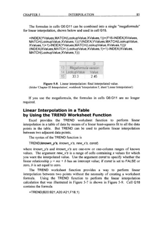
Figure 5-8. Linear interpolation: final interpolated value.
(folder 'Chapter 05 Interpolation', workbook 'Interpolation I', sheet 'Linear Interpolation')

If you use the megaformula, the formulas in cells G6:Gll are no longer
required.

Linear Interpolation in a Table
by Using the TREND Worksheet Function
Excel provides the TREND worksheet function to perform linear
interpolation in a table of data by means of a linear least-squares fit to all the data
points in the table. But TREND can be used to perform linear interpolation
between two adjacent data points.
The syntax of the TREND function is
TREND( knownj's, known-x's, new-x 's, consf)

where known-y's and known-x's are one-row or one-column ranges of known
values. The argument new-x's is a range of cells containing x values for which
you want the interpolated value. Use the argument consf to specify whether the
linear relationship y = mx + b has an intercept value; if const is set to FALSE or
zero, b is set equal to zero.
The TREND worksheet function provides a way to perform linear
interpolation between two points without the necessity of creating a worksheet
formula. Using the TREND function to perform the linear interpolation
calculation that was illustrated in Figure 5-7 is shown in Figure 5-9. Cell GI8
contains the formula

=TREND( 620: 62 I ,A20:A21, F18,l)