Page 244 - Excel for Scientists and Engineers: Numerical Methods

CHAPTER 10 ORDINARY DIFFERENTIAL EOUATIONS. PART I 22 1

( 10- 12)

(10-13)

(10-14)
(1 0- 15)

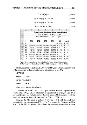
Figure 10-2. Simulation of first-order kinetics by the Runge-Kutta method.
(folder 'Chapter 10 Examples', workbook 'ODE Examples', worksheet 'MI')

The RK equations in cells 87, C7, D7, E7 and F7, respectively, are (only part
of the spreadsheet is shown; the formulas extend down to row 74):
=-k*FG*DX
=-k*( FG+TAl /2)*DX

=- k*( F6+TA2/2)*DX

=-k*( F6+TA3)*DX
=FG+(TAI +2*TA2+2*TA3+TA4)/6.
If you use the names TA1, . . ., TA4 you can use AutoFill to generate the
column labels TA1, . . ., TA4. These names are accepted by Excel, whereas T1 is
not a valid name. As well, the nomenclature is expandable to systems requiring
more than one set of Runge-Kutta terms (e.g., TB1, . . ., TB4, etc.).
Compare the RK result in column F of Figure 10-2 with the analytical
expression for the concentration, [A]t = in column G. After one half-life
(row 13) the RK calculation differs from the analytical expression by only