
Page 242 - Excel for Scientists and Engineers: Numerical Methods
P. 242
CHAPTER 10 ORDINARY DIFFERENTIAL EOUATIONS. PART I 219
The differential equation for the change in concentration of the species A as a
function of time is
d[ A] ldt = -k[ A] (1 0-4)
Expressing this in terms of finite differences, the change in concentration
A[A] that occurs during the time interval from t = 0 to t = At is
A[A] = -k[A], At (1 0-5)
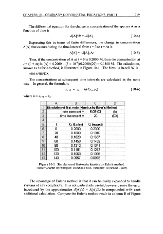
Thus, if the concentration of A at t = 0 is 0.2000 My then the concentration at
t = (0 + At) is [A] = 0.2000 - (5 x lO")(O.2OOO)(2O) = 0.1800 M. The calculation,
known as Euler's method, is illustrated in Figure 10-1. The formula in cell 87 is
=BG-k*BG*DX.
The concentrations at subsequent time intervals are calculated in the same
way. In general, the formula is
Yfl +I = Yfl + hF(x,,, Yfl) ( 10-6)
where h = xfl - x,.
Figure 10-1. Simulation of first-order kinetics by Euler's method.
(folder 'Chapter 10 Examples', workbook 'ODE Examples', worksheet 'Euler')
The advantage of Euler's method is that it can be easily expanded to handle
systems of any complexity. It is not particularly useful, however, since the error
introduced by the approximation d[A]ldt = A[A]/At is compounded with each
additional calculation. Compare the Euler's method result in column B of Figure