Page 134 - Fair, Geyer, and Okun's Water and wastewater engineering : water supply and wastewater removal

JWCL344_ch03_061-117.qxd 8/17/10 7:48 PM Page 96

96 Chapter 3 Water Sources: Groundwater

100

90

F p , percent of maximum specific capacity attainable
80

70

60
ABCDEFG b
Curve r w
50 A 40
B 60
C 80
40
D 100
E 120
30 F 200
G 400

20
b aquifer thickness
r w = well radius
10
Curves based on kozeny formula
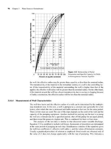
Figure 3.12 Relationship of Partial
0 10 20 30 40 50 60 70 80 90 100 Penetration and Specific Capacity for Wells
Percent of aquifer screened in Homogeneous Artesian Aquifers

the well, the effective radius may be greater than, equal to, or less than the nominal radius.
The transmissivity of the material in the immediate vicinity of a well is the controlling fac-
tor. If the transmissivity of the material surrounding the well is higher than that of the
aquifer, the effective well radius will be greater than the nominal radius. On the other hand,
if the material around the well has a lower transmissivity due to caving or clogging because
of faulty construction, the effective radius will be less than the nominal radius.

3.14.4 Measurement of Well Characteristics
The well-loss factor and the effective radius of a well can be determined by the multiple-
step drawdown test. In this test, a well is pumped at a constant rate (generally for a few
hours), after which the rate is increased and held constant at that rate for the same period.
Three or four steps are used. The size of the steps depends on the yield of the well and the
capacity of the pumping equipment. Another method for carrying out the test is to pump
the well at a constant rate for a specified period, shut off the pump for an equal period,
and then restart the pump at a higher rate. This is continued for three or four steps.
The analysis of the test data is similar to that discussed under variable discharge.
Equation 3.34 is modified to include well losses. Increments of drawdown are determined
at the same period of pumping in each step. Simultaneous solution of the equations gives
the well-loss coefficient C, effective well radius r, and the values of formation constants.
Usually a graphical procedure of solution is employed. Good results are obtained only if
the value of C does not change appreciably with the rate of pumping. This indicates a