Page 202 - Fiber Bragg Gratings

4.8 Grating simulation 179

l
[10]. The outputs of the first matrix M are used as the input fields to
1
2
the second matrix, M , not necessarily identical to M . The process is
continued until an entire complex profile grating is modeled. This method
is capable of accurately simulating both strong and weak gratings, with
or without chirp and apodization. It has the advantage of handling a
single period of grating as the minimum unit length for the matrix in the
case when the period or amplitude is a slowly varying function of length.
In the following section, two methods, Rouard's and the T-matrix, will be
presented for simulating gratings of arbitrary profile and chirp.

4.8.2 Transfer matrix method
An analytical solution for a grating of length L g, with an arbitrary coupling
constant K(Z) and chirp A(z), is desirable but no simple form exists. The
variables cannot be separated since they collectively affect the transfer
function. In the T-matrix method, the coupled mode equations [for exam-
ple, Eq. (4.3.9)] are used to calculate the output fields of a short section
S1 1 of grating for which the three parameters are assumed to be constant.
Each may possess a unique and independent functional dependence on
the spatial parameter z. For such a grating with an integral number
of periods, the analytical solution results in the amplitude reflectivity,
transmission, and phase. These quantities are then used as the input
parameters for the adjacent section of grating of length SL 2 (not necessarily
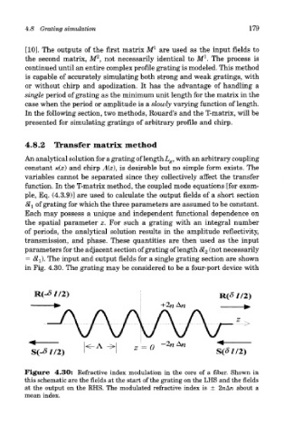
= 81 ±). The input and output fields for a single grating section are shown
in Fig. 4.30. The grating may be considered to be a four-port device with

Figure 4.30: Refractive index modulation in the core of a fiber. Shown in
this schematic are the fields at the start of the grating on the LHS and the fields
at the output on the RHS. The modulated refractive index is ± 2n&n about a
mean index.