Page 25 - Fiber Fracture

10 K.K. Chawla

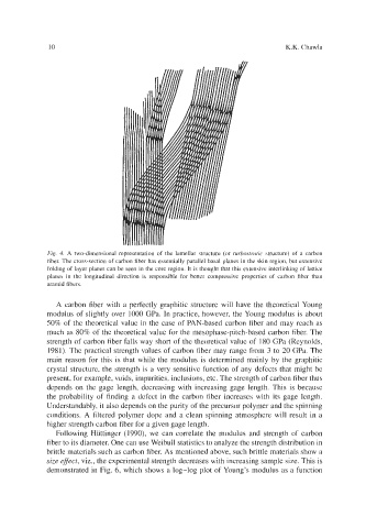
Fig. 4. A two-dimensional representation of the lamellar structure (or turbostrutic structure) of a carbon
fiber. The cross-section of carbon fiber has essentially parallel basal planes in the skin region, but extensive
folding of layer planes can be seen in the core region. It is thought that this extensive interlinking of lattice
planes in the longitudinal direction is responsible for better compressive properties of carbon fiber than
aramid fibers.

A carbon fiber with a perfectly graphitic structure will have the theoretical Young
modulus of slightly over 1000 GPa. In practice, however, the Young modulus is about
50% of the theoretical value in the case of PAN-based carbon fiber and may reach as
much as 80% of the theoretical value for the mesophase-pitch-based carbon fiber. The
strength of carbon fiber falls way short of the theoretical value of 180 GPa (Reynolds,
1981). The practical strength values of carbon fiber may range from 3 to 20 GPa. The
main reason for this is that while the modulus is determined mainly by the graphitic
crystal structure, the strength is a very sensitive function of any defects that might be
present, for example, voids, impurities, inclusions, etc. The strength of carbon fiber thus
depends on the gage length, decreasing with increasing gage length. This is because
the probability of finding a defect in the carbon fiber increases with its gage length.
Understandably, it also depends on the purity of the precursor polymer and the spinning
conditions. A filtered polymer dope and a clean spinning atmosphere will result in a
higher strength carbon fiber for a given gage length.
Following Hiittinger (1990), we can correlate the modulus and strength of carbon
fiber to its diameter. One can use Weibull statistics to analyze the strength distribution in
brittle materials such as carbon fiber. As mentioned above, such brittle materials show a
size eflect, viz., the experimental strength decreases with increasing sample size. This is
demonstrated in Fig. 6, which shows a log-log plot of Young’s modulus as a function