Page 340 - Fluid-Structure Interactions Slender Structure and Axial Flow (Volume 1)

320 SLENDER STRUCTURES AND AXIAL FLOW

(iii) In equation (5.107), F1 and F2 contain the still unknown Au and Ai. These are
determined by solving the differential equation in Au, equation (5.109, after the ‘modal
form’ of interest has been substituted in its right-hand side.
(iv) Now that all terms on the right-hand side of the reduced form of (5.103), equation
(5.106), are known, the nonlinear equation is solved by the Krylov-Bogoliubov method, a
form of averaging (Appendix F.4), keeping only the first term in the asymptotic expansion,
x = 0 sin 1c/ = i0 sin(wt + #), eventually leading to

(5.108)

where K1 and K2 are lengthy algebraic expressions involving the parameters in (5.107).
For a limit cycle, Oavg = 0; hence one obtains the limit-cycle amplitude

(5.109)

It is clear from (5.108) that the origin becomes unstable for a! > 0; furthermore, if K1 0
the emerging limit cycle is stable. On the other hand, if a! < 0 and K1 > 0, the limit cycle
is unstable.
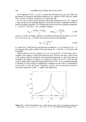
Typical results are shown in Figure 5.12. It is seen that for < 0.30 the limit cycle is
unstable, which suggests a subcritical Hopf bifurcation. However, the upper, stable branch
of the solution cannot be predicted, since polynomial expansions to only fourth order are
included in the analysis (cf. Section 2.3, Figures 2.12 and 2.13). For p > 0.30, the limit
cycle is stable and the Hopf bifurcation supercritical. For p = 0.30, an infinite amplitude
is obtained, but this should be interpreted as meaning that the effect of nonlinearities
(to the order to which the Krylov-Bogoliubov analysis and the polynomial expansions
have been carried out) is null - a higher order degeneracy.

1.25

1 .oo

2 0.75

0.50

0.25
, --Stable
Unstable L.C. - L.C. ---1
0
0 0.15 0.30 0.45
a

Figure 5.12 Limit-cycle amplitude, OLc, versus the mass ratio p, for an articulated cantilevered
system with c1 = c2 = 0, a = 1, h = 0.5, )Au,I = 0.1 (z 3%); (Rousselet & Herrmann 1977).