Page 32 - Fluid-Structure Interactions Slender Structure and Axial Flow (Volume 1)

CONCERTS, DEFINITIONS AND METHODS 15

sense, the ‘mix’ of first- and second-mode eigenfunctions of the original system, necessary
to approximate the eigenfunctions of the modified one; thus, for this example,

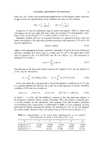
In general, N must be sufficiently large to assure convergence. Table 2.1 shows that
convergence can be very rapid. The exact values, by solving (2.22) with boundary condi-
tions (2.29), are f2r(EZ/mL4)-’/2 = 2.0163, 16.901,51.701 for r = 1,2, 3.
Galerkin’s method will now be expressed formally in a generalized form, useful for
further developrncnt. The eigenvalue problem associated with equations (2.22) and (2.30)
may be expressed as
Y[w] = AA[w], (2.36)

subject to the appropriate boundary conditions. Generally, 2 and A are linear differential
operators, although A in many cases is a scalar, and A(= Q2) is the eigenvalue. In the
case of equation (2.30), 3 = EI(a4/8x4) and A = m + M,S(x - L). The equivalent to
statement (2.31) now is
N
wN(x) = aj+j(x>. (2.37)
j= 1

The elements of the mass and stiffness matrices [cf. equation (2.1)], the two matrices in
(2.35), may be obtained by

(2.38)

In the case where Me is incorporated in A and the boundary conditions are (2.23), this
is a standard problem. If, however, M, is left out of the equations of motion, boundary
conditions (2.29) may be re-written as

w(0) = 0, w’(0) = 0, w”(L) = 0, EZw”’(L) = -hM,w(L), (2.39)

and
in which ( )’ = ?I/&, problem is unusual in that the eigenvalue appears in
the
the boundary conditions. Hence, strictly (Friedman 1956), the domain 9 depends upon
A. In this example, for the calculations with equation (2.22) and boundary conditions
(2.29) leading to the ‘exact results’ to which those of Table 2.1 were compared, we have
proceeded by blithely ignoring this subtlety (by retaining 9 = [0, l]), yet still obtained
the correct results. However, this is not always true, as will be seen in Section 2.1.4.

Table 2.1 Approximations to the lowest three eigenfrequencies of the modified
cantilevered pipe for various N in the case of M, = imL.
N 2 4 6 8 IO
RI (Ellm L4)-’I2 2.0 184 2.0166 2.0164 2.0163 2.0163
R2(El/m L4)-’I2 17.166 16.936 16.912 16.906 16.904
R3(El/m L4)-‘I2 - 52. I25 5 1.826 5 1.754 5 1.738