Page 35 - Fluid-Structure Interactions Slender Structure and Axial Flow (Volume 1)

18 SLENDER STRUCTURES AND AXIAL FLOW

2.1.6 Diagonalization, and forced vibrations of continuous systems
The equation of motion associated with the problem defined by (2.45) is
a4w a2w a2w
EI- +P- +m- =0, (2.47)
afi ax2 at2
with the boundary conditions as given in (2.46). This clearly represents free motions of the
system; hence, of interest are the eigenfrequencies and the corresponding eigenfunctions
and how they vary with P (or its nondimensional counterpart, PL2/EI). This can be
done by direct application of the Galerkin method with WN = Cj 4,(x)q,(t), in which
the cantilever-beam eigenfunctions (2.27) are used as comparison functions, since they
satisfy boundary conditions (2.46), which are identical to (2.23). In this way, one obtains
an equation similar to (2.35), i.e.

[MHii) + [KIM = IO)? (2.48)
but with only [MI being diagonal, while [K] is nondiagonal. In fact, the elements of
[K] are
L
k,, = EIk:LS,, + PI $,$;dx,

the prime denoting differentiation with respect to x.
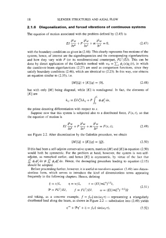
Suppose now that this system is subjected also to a distributed force, F(x, f), so that
the equation of motion is
a4w a2w a2w
EI-+P-+m- = F(x,t); (2.49)
ax4 ax2 at2
see Figure 2.2. After discretization by the Galerkin procedure, we obtain
[MIIii) + [KIkJ = {e). (2.50)

If this had been a self-adjoint conservative system, matrices [MI and [K] in equation (2.50)
would both be symmetric. For the problem at hand, however, the system is non-self-
adjoint, as remarked earlier, and hence [K] is asymmetric, by virtue of the fact that
@,# dx # 4,&! dx. Hence, the decoupling procedure leading to equation (2.15)
should be adopted.
Before proceeding further, however, it is useful to transform equation (2.49) into dimen-
sionless form, which serves to introduce the kind of dimensionless terms appearing
frequently in the following chapters. Hence, defining

= x/L, q = w/L, t = (EI/mL4)’/2t,
(2.5 1 )
8 = PL2/EI, f = FL3/EI, o = (EI/mL4)-’f2f2

and taking, as a concrete example, f = fo 6 sin (oft) - representing a triangularly
distributed load along the beam, as shown in Figure 2.2 - substitution into (2.49) yields

q”” + 9,’’ + ;i = fo 6 sin(wft), (2.52)