Page 33 - Fluid-Structure Interactions Slender Structure and Axial Flow (Volume 1)

16 SLENDER STRUCTURES AND AXIAL FLOW

2.1.4 Galerkin's method for a nonconservative system

Consider next that a fluid of constant velocity U and mass per unit length M is flowing
through the pipe in the example of Section 2.1.3, i.e. the pipe with the extra mass Me at
the free end. As shown in Chapter 3, the equation of motion in this case is

a4,v a2w a2w a2w
+
EI- +MU2 - +2MU - (m +M) - 0, (2.40)
=
ax4 ax2 axat at2
with boundary conditions (2.23) or (2.29) for Me = 0 and Me # 0, respectively.
For Me # 0, the problem is solved by the same two methods as before: (a) with Me
included in the equation of motion, with a Dirac delta function, and boundary conditions
(2.23); (b) with equation (2.40) as it stands and boundary conditions (2.29). Table 2.2
gives the results for r = M,/[(rn + M)L] = 0.3 and B M/(m + M) = 0.1 for two
values of the dimensionless flow velocity u = (M/IYI)'/~LU. Two interesting observa-
tions may be made from the results of Table 2.2. First, for u = 2, the eigenfrequencies
are no longer real; in fact, for all u # 0 they need not be real because the system is noncon-
servative. Second, the eigenfrequencies for u = 2 (again, for all u # 0) as obtained by
the two methods are not identical as they should have been.
That the system is nonconservative may be assessed by calculating the rate of work
done by all the forces acting on the pipe. If it is zero, then there is no net energy flow
in and out of the system, which must therefore be conservative; otherwise, the system is
nonconservative. In this case,

dW
dt (2.41)
is found not to be zero by virtue of the forces represented by the second and third terms in
(2.40)+ - see Chapter 3. Viewed another way, this means that it is not possible to derive
these forces from a potential; like dissipative forces, for instance, they are nonconservative,
at least for this set of boundary conditions.
The second observation suggests that, for u # 0, the results from either method (a) or
(b) must be wrong. Indeed, those of method (b), utilizing equations (2.40) and (2.29) as
they stand, are wrong because of the remark made at the end of Section 2.1.3. There is

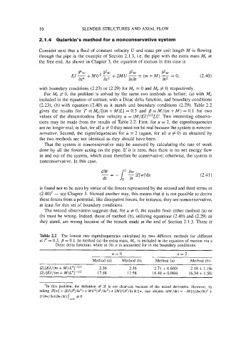
Table 2.2 The lowest two eigenfrequencies calculated by two different methods for different
u; r = 0.3, /3 = 0.1. In method (a) the extra mass, Me, is included in the equation of motion via a
Dirac delta function, while in (b) it is accounted for in the boundary conditions.
u=o I1 = 2
Method (a) Method (b) Method (a) Method (b)
R1 [EI/(m + M) L4]-'l2 2.36 2.36 2.7 1 + 0.660i 2.18+ 1.16i
Rz [EI/(m + M)L4]-1/2 17.58 17.58 16.48 + 0.084i 16.34 + 1.56i

+In this problem, the definition of Y is not clear-cut, because of the mixed derivative. However, by
taking ~[wI = [E1(#/ax4) + MU2(a2/ax2) + 2MU(a2/ax ar)]w, one obtains (dW/dt) = -MU[(aw/at)2 +
u(aw/ax)(wat)l/ X=L # 0.