Page 38 - Fluid-Structure Interactions Slender Structure and Axial Flow (Volume 1)

CONCEPTS, DEFINITIONS AND METHODS 21

in Figure 2.3(b), obtained with N = 1. A higher frequency component, at 01, is now
superposed on the solution. Two observations should be made: (i) since, unrealistically,
there is no damping in the system, the effect of initial conditions persists in perpetuity,
whereas, with even a small amount of damping, the steady-state response would be like
that in Figure 2.3(a); (ii) since q/wf is not rational, the response is not periodic but
quasiperiodic, although the effect of ‘unsteadiness’ in the response time-trace is just
barely visible. This is more pronounced in Figure 2.3(c), plotted on an expanded time-
scale, showing calculations with N = 2 and N = 4; in the latter case, the contribution of
all four eigenmodes is visible. On the other hand, the period associated with the forcing
frequency is hardly discernible in the time-scale used in Figure 2.3(c).
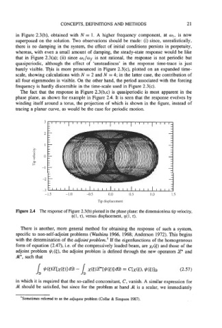
The fact that the response in Figure 2.3(b,c) is quasiperiodic is most apparent in the
phase plane, as shown for example in Figure 2.4. It is seen that the response evolves by
winding itself around a torus, the projection of which is shown in the figure, instead of
tracing a planar curve, as would be the case for periodic motion.

Figure 2.4 The response of Figure 2.3(b) plotted in the phase plane: the dimensionless tip velocity,
rj( 1, t), versus displacement, q( 1, t).

There is another, more general method for obtaining the response of such a system,
specific to non-self-adjoint problems (Washizu 1966, 1968; Anderson 1972). This begins
with the determination of the adjoint problem.+ If the eigenfunctions of the homogeneous
form of equation (2.47), Le. of the compressively loaded beam, are xi(t) and those of the
adjoint problem +;(e), the adjoint problem is defined through the new operators e* and
Y*, such that

(2.57)

in which it is required that the so-called concomitant, C, vanish. A similar expression for
M should be satisfied, but since for the problem at hand Y is a scalar, we immediately

‘Sometimes referred to as the adjugate problem (Collar & Simpson 1987).