Page 40 - Fluid-Structure Interactions Slender Structure and Axial Flow (Volume 1)

CONCEPTS, DEFINITIONS AND METHODS 23

2.2 THE FLUID MECHANICS OF FLUID-STRUCTURE
INTERACTIONS

2.2.1 General character and equations of fluid flow
Trying to give a selective encapsulation of the ‘fluids’ side of fluid-structure interactions
is more challenging than the equivalent effort on the ‘structures’ side, as attempted in
Section 2.1. Solution of the equations of motion of the fluid is much more difficult.
The equations are in most cases inherently nonlinear, for one thing; moreover, unlike
the situation in solid mechanics, linearization is not physically justifiable in many cases,
and solution of even the linearized equations is not trivial. Thus, complete analytical and,
despite the vast advances in computational fluid dynamic (CFD) techniques and computing
power, complefe numerical solutions are confined to only some classes of problems.
Consequently, there exists a large set of approximations and specialized techniques for
dealing with different types of problems, which is at the root of the difficulty remarked
at the outset. The interested reader is referred to the classical texts in fluid dynamics [e.g.
Lamb (1957), Milne-Thomson (1949, 1958), Prandtl (1952), Landau & Lifshitz (1959),
Schlichting (1960)] and more modem texts [e.g. Batchelor (1967), White (1 974), Hinze
(1975), Townsend (1976), Telionis (1981)l; a wonderful refresher is Tritton’s (1988) book.
Excluding non-Newtonian, stratified, rarefied, multi-phase and other ‘unusual’ fluid
flows,+ the basic fluid mechanics is governed by the continuity (i.e. conservation of mass)
and the Navier-Stokes (Le. conservation of momentum) equations. For a homogeneous,
isothermal, incompressible fluid flow of constant density and viscosity, with no body
forces, these are given by
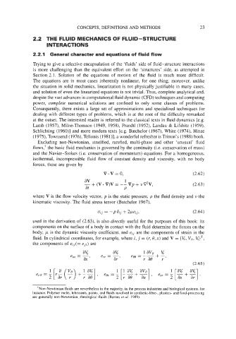
v.v=o, (2.62)
av 1
- + (V. V)V = -- vp+ vv*v, (2.63)
at P
where V is the flow velocity vector, p is the static pressure, p the fluid density and w the
kinematic viscosity. The fluid stress tensor (Batchelor 1967),

a;; = -pa;, + 2pe;j, (2.64)
used in the derivation of (2.63), is also directly useful for the purposes of this book: its
components on the surface of a body in contact with the fluid determine the forces on the
body; p is the dynamic viscosity coefficient, and e;; are the components of strain in the
fluid. In cylindrical coordinates, for example, where i, j = (r, 8, x) and V = {V, Vo, V,}T,
the components of e;j(= e;;) are
av, ar! 1 avo v
e, = - err = - em = -- + 2,
ax ’ ar ’ r a&’ r (2.65)
e,, = 2 [a, -4.
erH=T[rs(T)+;z], av, 1 av av,
a
+
1
1
v8
‘Non-Newtonian fluids are nevertheless in the majority, in the process industries and biological systems, for
instance. Polymer melts, lubricants, paints, and fluids involved in synthetic-fibre-, plastics- and food-processing
are generally non-Newtonian, rheological fluids (Barnes et al. 1989).