Page 124 - Fundamentals of Computational Geoscience Numerical Methods and Algorithms

112 5 Simulating Chemical Dissolution Front Instabilities in Fluid-Saturated Porous Rocks

∂C ∂p
= , 0 = 0
∂y ∂y
φ =φ f
C = C τ)( Inflow φφ
=
p ∂ = p′ o y L = 5
x ∂ fx C = 1
y

x
0
∂C ∂p
= , 0 = 0
∂y ∂y
x L = 10

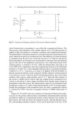
Fig. 5.1 Geometry and boundary conditions of the reactive infiltration problem

initial dimensionless-concentration is one within the computational domain. The
final porosity after depletion of the soluble mineral is 0.2. This final porosity is
applied on the left boundary as a boundary condition of the computational domain.
The permeability of the porous medium is calculated using the Carman-Kozeny for-
mula, which has the power of 3 in the power law. The diffusivity of chemical species
is calculated using the power law, which has the power of 2. Both the top and the
bottom boundaries are assumed to be impermeable for the pore-fluid and chemical
species. The ratio of the equilibrium concentration to the solid molar density of the
chemical species is assumed to be 0.01, while the dimensionless time-step is set
to be 0.005 in the computation. Since the computational domain of the benchmark
problem is of finite size, a time-dependent-dimensionless-concentration boundary
condition (i.e. C(τ) = exp(p ν front τ)) needs to be applied on the left boundary so

fx
that the numerical solutions can be compared with the analytical solutions derived
in the previous section. Using the above-mentioned parameters, the critical Zhao
number of the system is approximately equal to 1.77. Since the Zhao number of
the system is smaller than its critical value, the coupled system considered in this
section is sub-critical so that a planar dissolution front remains planar during its
propagation within the system. The dimensionless speed of the dissolution front
propagation is equal to 10, which is determined using Eq. (5.51). To simulate appro-
priately the propagation of the dissolution front, the whole computational domain
is simulated by 19701 four-node rectangular elements of 20000 nodal points in
total.
Figures 5.2, 5.3 and 5.4 show the comparison of numerical solutions with analyt-
ical ones for the porosity, dimensionless concentration and dimensionless pressure
distributions within the computational domain at three different time instants. In
these figures, the thick line shows the numerical results, while the thin line shows
the corresponding analytical solutions, which can be determined from Eqs. (5.49)