Page 125 - Fundamentals of Computational Geoscience Numerical Methods and Algorithms

5.2 Segregated Algorithm for Simulating the Morphological Evolution 113

0.2 0.2

Porosity Porosity

0.1 0.1
0 10 0 10
x x
(τ = 0.25) (τ = 0.625)

0.2

Porosity

0.1
0 10
x
(τ = 0.8)

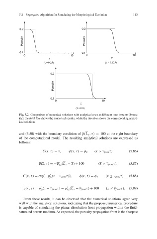
Fig. 5.2 Comparison of numerical solutions with analytical ones at different time instants (Poros-
ity): the thick line shows the numerical results, while the thin line shows the corresponding analyt-
ical solutions

and (5.50) with the boundary condition of p(L x ,τ) = 100 at the right boundary
of the computational model. The resulting analytical solutions are expressed as
follows:

C(x,τ) = 1, φ(x,τ) = φ 0 (x > ν front τ), (5.86)

p(x,τ) =−p (L x − x) + 100 (x > ν front τ), (5.87)
0x

C(x,τ) = exp[−p (x − ν front τ)], (x ≤ ν front τ), (5.88)
fx φ(x,τ) = φ f

p(x,τ) = p (x − ν front τ) − p (L x − ν front τ) + 100 (x ≤ ν front τ). (5.89)
fx
0x
From these results, it can be observed that the numerical solutions agree very
well with the analytical solutions, indicating that the proposed numerical procedure
is capable of simulating the planar dissolution-front propagation within the fluid-
saturated porous medium. As expected, the porosity propagation front is the sharpest