Page 299 - Fundamentals of Gas Shale Reservoirs

UPSCALING HETEROGENEOUS SHALE‐GAS RESERVOIRS INTO LARGE HOMOGENIZED SIMULATION GRID BLOCKS 279
As stated earlier, the actual distribution of and the volume
1.0 Continuum model occupied by the quad‐porosity subsystems in shale are usu­
Recovery factor, fraction 0.6 distributions in a manner to preserve the total porosity of
0.8
Tank model
ally not known. This problem can be alleviated by random
each subsystem. A second reason for using a random model
is for systems that combine very low permeability storage
0.4
units with high permeability transport units in upscaling is
0.2
an average sense be preserved. If one just takes a pattern of
0.0 the time it takes fluid to flow into the transport units must in
units and magnifies all the distances without making any
–1.0 0.0 1.0 2.0 3.0 4.0 other changes, then the production curve will not be pre­
Log (time, days) served. Certain prescribed organic pattern distributions are
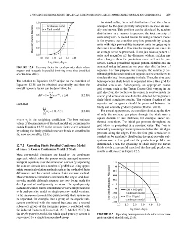
FIGURE 12.4 Recovery factor for quad‐porosity shale where assumed using information on pore size distributions of
organic and inorganic in parallel involving cross flow (modified organics. For this purpose, for example, the randomly dis­
after Hudson, 2013). tributed globules and streaks of organic can be considered to
simulate the local heterogeneity in shale. Then, the simulated
The solution to Equation 12.37 subject to the condition of heterogeneous shale block is separated into a fine grid for
Equation 12.38 can be obtained analytically and then the detailed simulation. Subsequently, an appropriate coarse
overall recovery factor can be determined by grid system, such as the Tartan Coarse Grid varying in the
N 4 grid size from the borders to the center, is used to match the
RF 1 we t i t , 0 (12.39) coarse grid simulation results to the detailed heterogeneous
i 1 i shale block simulation results. The volume fraction of the

Such that organics and inorganics should be preserved between the
finely and coarsely gridded systems (Michel, 2013).
N 4
w 10., t 0 (12.40) For upscaling purposes, we consider simulating the flow
i 1 i of only the methane gas phase through the shale over a
square domain of unit thickness, for example, under iso­
where w is the weighting coefficient. The best estimate
i
values of the parameters of the tank model are determined to thermal conditions. The initial gas pressure throughout the
match Equation 12.37 to the recover factor curve obtained grid block is prescribed at a constant value. The flow is
by solving the finely gridded reservoir block as described in induced by assuming constant pressures below the initial gas
the next section (Fig. 12.4). pressure along the edges. First, the fine grid simulation is
carried out by randomly distributing the quad‐porosity sub­
systems over a fine grid and the production profiles are
determined. Then, the upscaling of shale using the Tartan
12.7.2 Upscaling Finely Detailed Continuum Model Grids yields a successful match of the fine‐grid production
of Shale to Coarse Continuum Model of Shale
results as illustrated in Figure 12.5.
Most commercial simulators are based on the continuum
approach, which solve the porous media averaged reservoir
transport equations over the simulation domain by separating 1.5
the solution domain into a number of grid blocks using appro­ 1.0
priate numerical solution methods such as the method of finite 0.5
differences and the control volume finite element method.
Most commercial simulators can handle the single‐ and dual‐ 0.0
porosity models although attempts are now being made for log (production rate, Mscf/day) –0.5
development of multiporosity versions. The quad‐porosity –1.5
system sometimes can be simulated after some simplifications –1.0 100 × 100 grid
with dual‐porosity model or single‐porosity model versions. –2.0 continuum model
In the dual‐porosity model the quad‐porosity shale system can 10 × 10 grid
be separated, for example, into a group of the organic sub­ –2.5 continuum model
system combined with the natural fractures and a second –3.0
subsystem group of the inorganic porosity combined with 0.0 1.0 2.0 3.0 4.0 5.0
the induced fractures (Civan et al., 2013; Michel, 2013). In log (time, days)
the single‐porosity model, the whole quad‐porosity system is FIGURE 12.5 Upscaling heterogeneous shale with tartan coarse
represented by a single homogenized group. grids (modified after Michel, 2013).