Page 192 - Fundamentals of Geomorphology

HILLSLOPES 175

substitution allows the reconstruction of long-term from the watershed (roughly the distance of overland
n
changes in hillslopes under special circumstances (p. 25). flow) and (dh/dx) represents processes in which sedi-
Mathematical models offer another means of probing ment transport is proportional to slope gradient. Empir-
m
long-term changes in hillslope form. ical work suggests that f (x) m = x , where m varies
Michael J. Kirkby is a leading figure in the field of according to the sediment-moving processes in opera-
hillslope modelling. He used the continuity equation tion, representative values being 0 for soil creep and
of debris moving on hillslopes and in rivers as a basis for rainsplash and 1.3–1.7 for soil wash. The exponent n
hillslope models (Kirkby 1971). In one dimension, the is typically 1.0 for soil creep, 1.0–2.0 for rainsplash,
equation of debris on a hillside is: and 1.3–2.0 for soil wash (Kirkby 1971). For a hill-
slope catena, the solution of the equation takes the
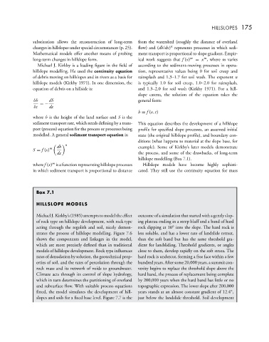
δh dS general form:
=−
δt dx
h = f (x, t)
where h is the height of the land surface and S is the
sediment transport rate, which needs defining by a trans- This equation describes the development of a hillslope
port (process) equation for the process or processes being profile for specified slope processes, an assumed initial
modelled. A general sediment transport equation is: state (the original hillslope profile), and boundary con-
ditions (what happens to material at the slope base, for
dh n example). Some of Kirkby’s later models demonstrate
S = f (x) m
dx the process, and some of the drawbacks, of long-term
hillslope modelling (Box 7.1).
m
where f (x) is a function representing hillslope processes Hillslope models have become highly sophisti-
in which sediment transport is proportional to distance cated. They still use the continuity equation for mass

Box 7.1

HILLSLOPE MODELS

Michael J. Kirkby’s (1985) attempts to model the effect outcome of a simulation that started with a gently slop-
of rock type on hillslope development, with rock type ing plateau ending in a steep bluff and a band of hard
acting through the regolith and soil, nicely demon- rock dipping at 10 into the slope. The hard rock is
◦
strates the process of hillslope modelling. Figure 7.6 less soluble, and has a lower rate of landslide retreat,
shows the components and linkages in the model, than the soft band but has the same threshold gra-
which are more precisely defined than in traditional dient for landsliding. Threshold gradients, or angles
models of hillslope development. Rock type influences close to them, develop rapidly on the soft strata. The
rates of denudation by solution, the geotechnical prop- hard rock is undercut, forming a free face within a few
erties of soil, and the rates of percolation through the hundred years. After some 20,000 years, a summit con-
rock mass and its network of voids to groundwater. vexity begins to replace the threshold slope above the
Climate acts through its control of slope hydrology, hard band, the process of replacement being complete
which in turn determines the partitioning of overland by 200,000 years when the hard band has little or no
and subsurface flow. With suitable process equations topographic expression. The lower slope after 200,000
fitted, the model simulates the development of hill- years stands at an almost constant gradient of 12.4 ,
◦
slopes and soils for a fixed base level. Figure 7.7 is the just below the landslide threshold. Soil development