Page 178 - Fundamentals of Ocean Renewable Energy Generating Electricity From The Sea

In Situ and Remote Methods for Resource Characterization Chapter | 7 167

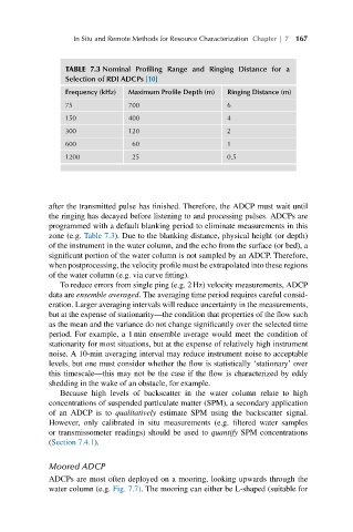
TABLE 7.3 Nominal Profiling Range and Ringing Distance for a
Selection of RDI ADCPs [10]
Frequency (kHz) Maximum Profile Depth (m) Ringing Distance (m)
75 700 6
150 400 4
300 120 2
600 60 1
1200 25 0.5

after the transmitted pulse has finished. Therefore, the ADCP must wait until
the ringing has decayed before listening to and processing pulses. ADCPs are
programmed with a default blanking period to eliminate measurements in this
zone (e.g. Table 7.3). Due to the blanking distance, physical height (or depth)
of the instrument in the water column, and the echo from the surface (or bed), a
significant portion of the water column is not sampled by an ADCP. Therefore,
when postprocessing, the velocity profile must be extrapolated into these regions
of the water column (e.g. via curve fitting).
To reduce errors from single ping (e.g. 2 Hz) velocity measurements, ADCP
data are ensemble averaged. The averaging time period requires careful consid-
eration. Larger averaging intervals will reduce uncertainty in the measurements,
but at the expense of stationarity—the condition that properties of the flow such
as the mean and the variance do not change significantly over the selected time
period. For example, a 1 min ensemble average would meet the condition of
stationarity for most situations, but at the expense of relatively high instrument
noise. A 10-min averaging interval may reduce instrument noise to acceptable
levels, but one must consider whether the flow is statistically ‘stationary’ over
this timescale—this may not be the case if the flow is characterized by eddy
shedding in the wake of an obstacle, for example.
Because high levels of backscatter in the water column relate to high
concentrations of suspended particulate matter (SPM), a secondary application
of an ADCP is to qualitatively estimate SPM using the backscatter signal.
However, only calibrated in situ measurements (e.g. filtered water samples
or transmissometer readings) should be used to quantify SPM concentrations
(Section 7.4.1).

Moored ADCP
ADCPs are most often deployed on a mooring, looking upwards through the
water column (e.g. Fig. 7.7). The mooring can either be L-shaped (suitable for