Page 122 - Fundamentals of Probability and Statistics for Engineers

Expectations and Moments 105

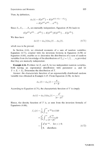
Then, by definition,
Y t†ˆ Efe jtY gˆ Efe jt X 1 ‡X 2 ‡ ‡X n † g
ˆ Efe jtX 1 jtX 2 ... e jtX n g:
e
Since X 1 , X 2 ,..., X n are mutually independent, Equation (4.36) leads to

Efe jtX 1 jtX 2 ... e jtX n gˆ Efe jtX 1 gEfe jtX 2 g ... Efe jtX n g:
e
We thus have
t†; 4:71†
Y t†ˆ X 1 t† X 2 t† ... X n
which was to be proved.
In Section (4.4), we obtained moments of a sum of random variables;
Equation (4.71), coupled with the inversion formula in Equation (4.58) or
Equation (4.64), enables us to determine the distribution of a sum of random
variables from the knowledge of the distributions of X j , j ˆ 1, 2, .. . , n, provided
that they are mutually independent.

Example 4.16. Problem: let X 1 and X 2 be two independent random variables,

both having an exponential distribution with parameter a, and let
Y ˆ X 1 ‡ X 2 . Determine the distribution of Y .
Answer: the characteristic function of an exponentially distributed random
variable was obtained in Example 4.15. From Equation (4.54), we have
a
t†ˆ :
X 1 t†ˆ X 2
a jt
According to Equation (4.71), the characteristic function of Y is simply

a 2
t†ˆ :
Y t†ˆ X 1 t† X 2 2
a jt†
Hence, the density function of Y is, as seen from the inversion formula of
Equations (4.68),
1 Z 1
f y†ˆ e jty Y t†dt
Y
2 1
a 2 Z 1 e jty
ˆ dt
2 1 a jt† 2
2 ay
a ye ; for y 0;
ˆ 4:72†
0; elsewhere:

TLFeBOOK