Page 120 - Fundamentals of Probability and Statistics for Engineers

Expectations and Moments 103

However, notice that, since X is continuous, P(X ˆ x) ˆ 0 if x is a point of
continuity in the distribution of X. Hence, using Equation (4.47),

EfYgˆ P X < x†ˆ F X x†

1 j Z 1 1 Efe j X x†t g
ˆ dt 4:62†
2 2 1 t

1 j Z 1 1 e jtx X t†
ˆ dt:
2 2 1 t
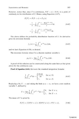
The above defines the probability distribution function of X. Its derivative
gives the inversion formula

1 Z 1 jtx
f x†ˆ e X t†dt; 4:63†
X 2 1
and we have Equation (4.58), as desired.

The inversion formula when X is a discrete random variable is
1 Z u
p x†ˆ lim e jtx X t†dt: 4:64†
X
u!1 2u
u
A proof of this relation can be constructed along the same lines as that given
above for the continuous case.

Proof of Equation (4.64): first note the standard integration formula:

sin au
8
u
1 Z jat < ; for a 6ˆ 0;
e dt ˆ au 4:65†
2u u :
1; for a ˆ 0:

Replacing a by X x and taking the limit as u !1, we have a new random
variable Y , defined by

1 Z u j X x†t 0; for X 6ˆ x;
Y ˆ lim e dt ˆ
u!1 2u
u 1; for X ˆ x:
The mean of Y is given by

EfYgˆ 1†P X ˆ x†‡ 0†P X 6ˆ x†ˆ P X ˆ x†; 4:66†

TLFeBOOK