Page 137 - Fundamentals of Probability and Statistics for Engineers

120 Fundamentals of Probability and Statistics for Engineers

where g(X ) is assumed to be a continuous function of X. Given the probability
distribution of X in terms of its probability distribution function (PDF),
probability mass function (pmf ) or probability density function (pdf ), we
are interested in the corresponding distribution for Y and its moment
properties.

5.1.1 PROBABILITY DISTRIBUTION

Given the probability distribution of X, the quantity Y , being a function of X as
defined by Equation (5.2), is thus also a random variable. Let R X be the range
space associated with random variable X, defined as the set of all possible
values assumed by X, and let R Y be the corresponding range space associated
with Y . A basic procedure of determining the probability distribution of Y
consists of the steps developed below.
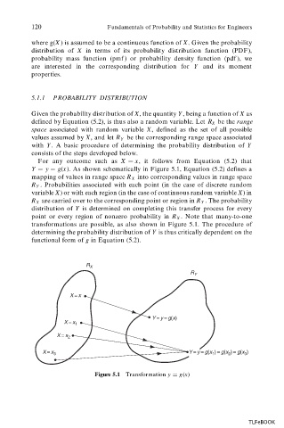
For any outcome such as X ˆ x, it follows from Equation (5.2) that
Y ˆ y ˆ g(x). As shown schematically in Figure 5.1, Equation (5.2) defines a
mapping of values in range space R X into corresponding values in range space
R Y . Probabilities associated with each point (in the case of discrete random
variable X) or with each region (in the case of continuous random variable X) in
R X are carried over to the corresponding point or region in R Y . The probability
distribution of Y is determined on completing this transfer process for every
point or every region of nonzero probability in R X . Note that many-to-one
transformations are possible, as also shown in Figure 5.1. The procedure of
determining the probability distribution of Y is thus critically dependent on the
functional form of g in Equation (5.2).

R X
R Y

X = x

Y = y = g(x)
X = x 1
X = x 2

X = x 3 Y = y = g(x )= g(x )= g(x )
1
3
2

Figure 5.1 Transformation y ˆ g(x)

TLFeBOOK