Page 180 - Fundamentals of Probability and Statistics for Engineers

Some Important Discrete Distributions 163

where
n
n!
ˆ 6:3†
k k! n k†!
is the binomial coefficient in the binomial theorem

n
n
n X k n k
a ‡ b† ˆ a b : 6:4†
k
kˆ0
In view of its similarity in appearance to the terms of the binomial theorem,
the distribution defined by Equation (6.2) is called the binomial distribution.
It has two parameters, namely, n and p. Owing to the popularity of this
distribution, a random variable X having a binomial distribution is often
denoted by B(n, p).
The shape of a binomial distribution is determined by the values assigned
to its two parameters, n and p. In general, n is given as a part of the problem
statement and p must be estimated from observations.
A plot of probability mass function (pmf), p X (k), has been shown in Example
3.2 (page 43) for n ˆ 10 and p ˆ 0.2. The peak of the distribution will shift to
the right as p increases, reaching a symmetrical distribution when p ˆ 0.5. More
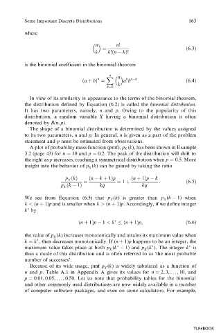
insight into the behavior of p (k) can be gained by taking the ratio
X
p k† n k ‡ 1†p n ‡ 1†p k
X
p k 1† ˆ kq ˆ 1 ‡ kq : 6:5†
X
We see from Equation (6.5) that p (k) is greater than p (k 1) when
X
X
k < (n ‡ 1)p and is smaller when k > (n ‡ 1)p. Accordingly, if we define integer

k by

n ‡ 1†p 1 < k n ‡ 1†p; 6:6†
the value of p (k) increases monotonically and attains its maximum value when
X

k ˆ k , then decreases monotonically. If (n ‡ 1)p happens to be an integer, the

maximum value takes place at both p (k 1) and p (k ). The integer k is
X
X
thus a mode of this distribution and is often referred to as ‘the most probable
number of successes’.
Because of its wide usage, pmf p (k) is widely tabulated as a function of
X
n and p. Table A.1 in Appendix A gives its values for n ˆ 2, 3, . . . , 10, and
p ˆ 0.01, 0.05, .. . , 0.50. Let us note that probability tables for the binomial
and other commonly used distributions are now widely available in a number
of computer software packages, and even on some calculators. For example,

TLFeBOOK