Page 228 - Fundamentals of Probability and Statistics for Engineers

Some Important Continuous Distributions 211

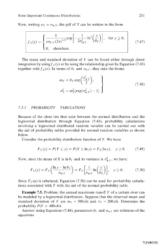
Now, writing X ˆ ln Y , the pdf of Y can be written in the form

8
1 1 2 y
> exp ln ; for y 0;
< 1=2 2
f y†ˆ y ln Y 2 † 2 ln Y Y 7:47†
Y
>
0; elsewhere:
:
The mean and standard deviation of Y can be found either through direct
integration by using f (y) or by using the relationship given by Equation (7.43)
Y

together with f (x). In terms of Y and ln Y , they take the forms
X
2 9
ln Y
m Y ˆ Y exp ; >
>
=
2 7:48†
>
2
2
>
ˆ m ‰exp 2 † 1Š: ;
Y Y ln Y
7.3.1 PROBABILITY TABULATIONS
Because of the close ties that exist between the normal distribution and the
lognormal distribution through Equation (7.43), probability calculations
involving a lognormal distributed random variable can be carried out with
the aid of probability tables provided for normal random variables as shown
below.
Consider the probability distribution function of Y . We have
F Y y†ˆ P Y y†ˆ P X ln y†ˆ F X ln y†; y 0: 7:49†

Now, since the mean of X is ln Y and its variance is 2 ln Y , we have:

ln y ln Y 1 y
F Y y†ˆ F U ˆ F U ln ; y 0: 7:50†
ln Y ln Y Y
Since F U (u) is tabulated, Equation (7.50) can be used for probability calcula-
tions associated with Y with the aid of the normal probability table.
Example 7.5. Problem: the annual maximum runoff Y of a certain river can

be modeled by a lognormal distribution. Suppose that the observed mean and
standard deviation of Y are m Y ˆ 300 cfs and ˆ 200 cfs. Determine the
Y
probability P(Y > 400 cfs).
Answer: using Equations (7.48), parameters Y and ln Y are solutions of the

equations

TLFeBOOK