Page 226 - Fundamentals of Probability and Statistics for Engineers
P. 226
Some Important Continuous Distributions 209
7.3 LOGNORMAL DISTRIBUTION
We have seen that normal distributions arise from sums of many random
actions. Consider now another common phenomenon which is the resultant
of many multiplicative random effects. An example of multiplicative phenom-
ena is in fatigue studies of materials where internal material damage at a given
stage of loading is a random proportion of damage at the previous stage. In
biology, the distribution of the size of an organism is another example for
which growth is subject to many small impulses, each of which is proportional
to the momentary size. Other examples include the size distribution of particles
under impact or impulsive forces, the life distribution of mechanical compon-
ents, the distribution of personal incomes due to annual adjustments, and other
similar phenomena.
Let us consider
Y X 1 X 2 ... X n :
7:41
We are interested in the distribution of Y as n becomes large, when random
variables X j , j 1, 2, .. ., n, can take only positive values.
If we take logarithms of both sides, Equation (7.41) becomes
ln Y ln X 1 ln X 2 ln X n :
7:42
The random variable ln Y is seen as a sum of random variables ln X 1 , ln X 2 ,. . . ,
and ln X n . It thus follows from the central limit theorem that ln Y tends to
a normal distribution as n !1. The probability distribution of Y is thus
determined from
X
Y e ;
7:43
where X is a normal random variable.
Definition 7.1. Let X be N(m X , 2 X ). The random variable Y as determined
from Equation (7.43) is said to have a lognormal distribution.
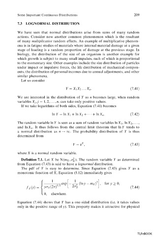
The pdf of Y is easy to determine. Since Equation (7.43) gives Y as a
monotonic function of X, Equation (5.12) immediately gives
1 1 2
8
> exp
ln y m X ; for y 0;
< 1=2 2
f
y y X
2 2 X
7:44
Y
>
:
0; elsewhere:
Equation (7.44) shows that Y has a one-sided distribution (i.e. it takes values
only in the positive range of y). This property makes it attractive for physical
TLFeBOOK

