Page 364 - Fundamentals of Probability and Statistics for Engineers

Linear Models and Linear Regression 347

Answer: in this case, we have n ˆ 14. The quantities of interest are
n
1 X 1
x ˆ x i ˆ 2 ‡ 2:5 ‡ ‡ 20†ˆ 11:11;
n 14
iˆ1
n
1 X 1
y ˆ y i ˆ 9:1 ‡ 19:2 ‡ ‡ 130:8†ˆ 57:59;
n 14
iˆ1
n
X 2
x i x† ˆ 546:09;
iˆ1
n
X 2
y i y† ˆ 17; 179:54;
iˆ1
n
X
x i x† y i y†ˆ 2862:12:
iˆ1
The substitution of these values into Equations (11.7), (11.8), and (11.33) gives
^
ˆ 2862:12 ˆ 5:24;
546:09
^ ˆ 57:59 5:24 11:11†ˆ 0:63;
1 2
b 2
ˆ ‰17; 179:54 5:24† 546:09†Š ˆ 182:10:
12
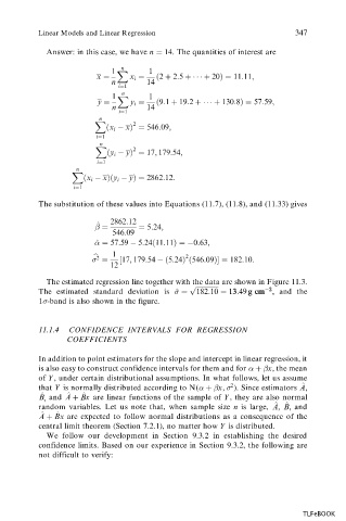
The estimated regression line together with the data are shown in Figure 11.3.
p
The estimated standard deviation is ^ ˆ  13 13 49 g cm 2 2 ,
:
182:10 ˆ
g cm ,and the

1 -band is also shown in the figure.
11.1.4 CONFIDENCE INTERVALS FOR REGRESSION
COEFFICIENTS

In addition to point estimators for the slope and intercept in linear regression, it
is also easy to construct confidence intervals for them and for ‡ x, the mean
of Y , under certain distributional assumptions. In what follows, let us assume
^
that Y is normally distributed according to N( ‡ x, 2 ). Since estimators A,
^
^
^
B, and A ‡ B x are linear functions of the sample of Y , they are also normal
^ ^
random variables. Let us note that, when sample size n is large, A, B, and
^
^
A ‡ Bx are expected to follow normal distributions as a consequence of the
central limit theorem (Section 7.2.1), no matter how Y is distributed.
We follow our development in Section 9.3.2 in establishing the desired
confidence limits. Based on our experience in Section 9.3.2, the following are
not difficult to verify:

TLFeBOOK