Page 366 - Fundamentals of Probability and Statistics for Engineers

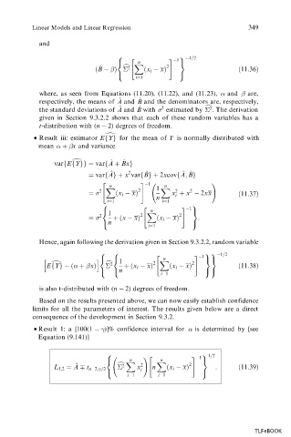
Linear Models and Linear Regression 349

and
1=2
8 9
" # 1
n
< X =
^
B † x i x† 2 11:36†
c 2
iˆ1
: ;
where, as seen from Equations (11.20), (11.22), and (11.23), and are,
respectively, the means of A ^ and ^ and the denominators are, respectively,
B
^
B
the standard deviations of A and ^ with 2 estimated by 2 c . The derivation
given in Section 9.3.2.2 shows that each of these random variables has a
t-distribution with (n 2) degrees of freedom.
. Result iii: estimator EfYg for the mean of Y is normally distributed with
d
mean ‡ x and variance
^
^
varfEfYgg ˆ varfA ‡ Bxg
d
^ ^
^
^
2
ˆ varfAg‡ x varfBg‡ 2xcovfA; Bg
" # 1 !
n
n 1 X
2
X
2
ˆ 2 x i x† 2 x ‡ x 2xx 11:37†
i
n
iˆ1 iˆ1
8 9
" # 1
1 2 X 2
< n =
2
ˆ ‡ x x† x i x† :
n
: ;
iˆ1
Hence, again following the derivation given in Section 9.3.2.2, random variable
8 8 99 1=2
" # 1
1 2 X 2
h i< < n ==
c 2
EfYg ‡ x† ‡ x i x† x i x† 11:38†
d
n
iˆ1
: : ;;
is also t-distributed with (n 2) degrees of freedom.
Based on the results presented above, we can now easily establish confidence
limits for all the parameters of interest. The results given below are a direct
consequence of the development in Section 9.3.2.
.Result 1: a [100(1
)]% confidence interval for is determined by [see
Equation (9.141)]
8 9 1=2
!" # 1
n n
< X X =
^ c 2 2 2
L 1;2 ˆ A t n 2;
=2 x n x i x† : 11:39†
i
iˆ1 iˆ1
: ;
TLFeBOOK