Page 190 - Fundamentals of Radar Signal Processing

so that the approximation R ≈ cT/2 from Eq. (3.9) can be used for simplicity.
ua
The same target echo profile is repeated, simply delayed by T seconds as shown
on the second line. The next line continues this behavior for a third pulse and
any subsequent pulses.

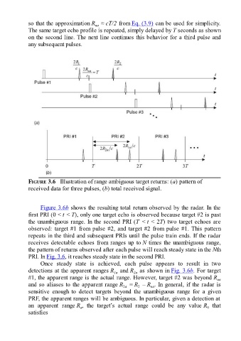
FIGURE 3.6 Illustration of range ambiguous target returns: (a) pattern of

received data for three pulses, (b) total received signal.

Figure 3.6b shows the resulting total return observed by the radar. In the

first PRI (0 < t < T), only one target echo is observed because target #2 is past
the unambiguous range. In the second PRI (T < t < 2T) two target echoes are
observed: target #1 from pulse #2, and target #2 from pulse #1. This pattern
repeats in the third and subsequent PRIs until the pulse train ends. If the radar
receives detectable echoes from ranges up to N times the unambiguous range,
the pattern of returns observed after each pulse will reach steady state in the Nth
PRI. In Fig. 3.6, it reaches steady state in the second PRI.

Once steady state is achieved, each pulse appears to result in two
detections at the apparent ranges R and R as shown in Fig. 3.6b. For target
1a
2a
#1, the apparent range is the actual range. However, target #2 was beyond R ua
and so aliases to the apparent range R = R – R . In general, if the radar is
2a
ua
2
sensitive enough to detect targets beyond the unambiguous range for a given
PRF, the apparent ranges will be ambiguous. In particular, given a detection at
an apparent range R , the target’s actual range could be any value R that
0
a
satisfies