Page 186 - Fundamentals of Radar Signal Processing

with a velocity spread of 110 mph, or about 50 m/s. For a more extreme

example, consider a moving radar installed on one of two subsonic (200 m/s)
jet aircraft flying in opposite directions. As they approach, the closing rate is
400 m/s; once they pass, they separate at 400 m/s. The change in velocities
observed by the radar on one of the aircraft over time is 800 m/s.
A moving radar can also induce a spread in the Doppler bandwidth of
stationary objects in the beam. This is most relevant in air-to-ground radars.

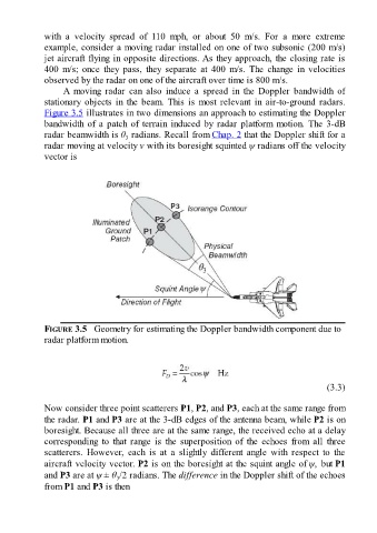
Figure 3.5 illustrates in two dimensions an approach to estimating the Doppler
bandwidth of a patch of terrain induced by radar platform motion. The 3-dB
radar beamwidth is θ radians. Recall from Chap. 2 that the Doppler shift for a
3
radar moving at velocity v with its boresight squinted ψ radians off the velocity
vector is

FIGURE 3.5 Geometry for estimating the Doppler bandwidth component due to
radar platform motion.

(3.3)

Now consider three point scatterers P1, P2, and P3, each at the same range from
the radar. P1 and P3 are at the 3-dB edges of the antenna beam, while P2 is on
boresight. Because all three are at the same range, the received echo at a delay
corresponding to that range is the superposition of the echoes from all three

scatterers. However, each is at a slightly different angle with respect to the
aircraft velocity vector. P2 is on the boresight at the squint angle of ψ, but P1
and P3 are at ψ ± θ /2 radians. The difference in the Doppler shift of the echoes
3
from P1 and P3 is then